Preface
Goal: A quick glance to the open source PSPPire.
I would really like to explore PSPPire. PSPP is the open source version of SPSS.
We need to verify the result of our previous excel and python, with a real statistic application.
Using PSPPire
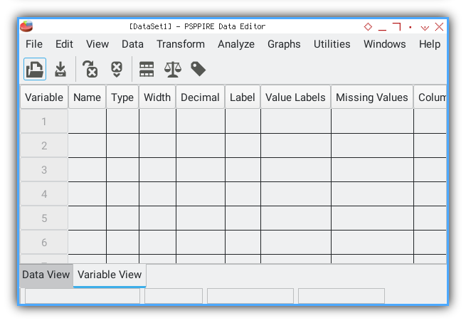
The first time using PSPPire is easy as long as you know this interface.
User Interface
The PSPP itself is just a TUI (terminal user interface).
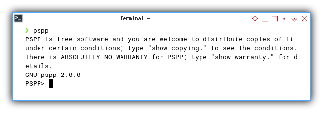
You need PSPPire to run the GUI (graphical user interface)
Import Data
We can import our previous CSV series using Import Data menu.
For example this CSV file
x, y
0, 5
1, 12
2, 25
3, 44
4, 69
5, 100
6, 137
7, 180
8, 229
9, 284
10, 345
11, 412
12, 485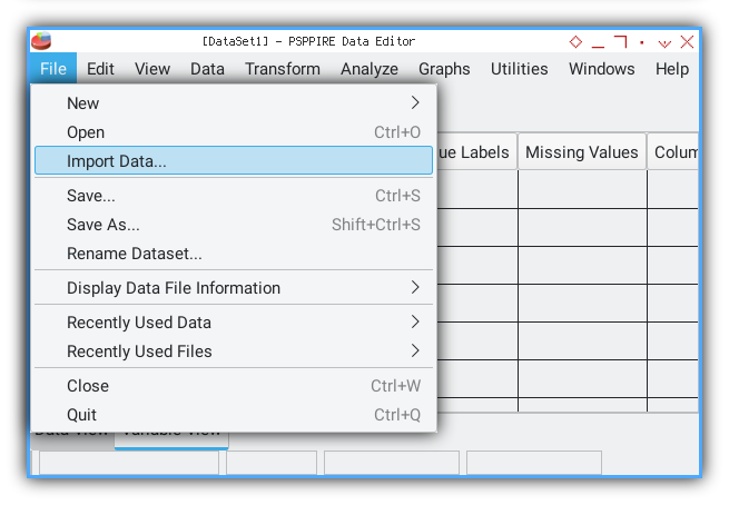
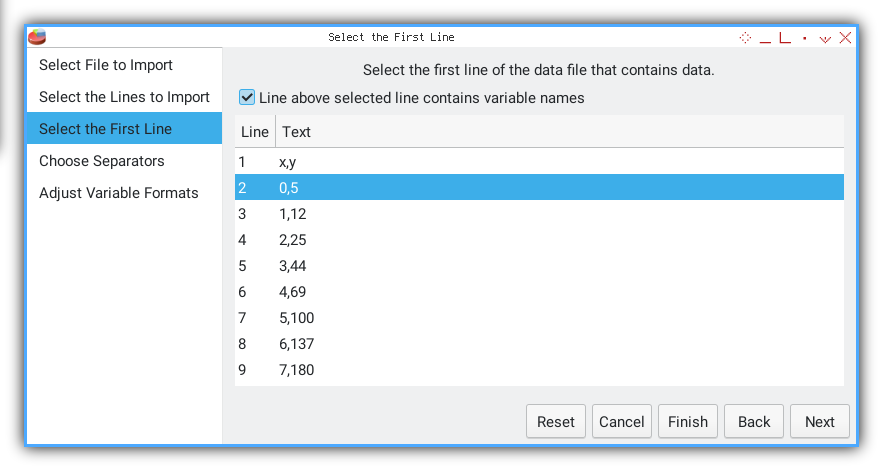
We need to follow required procedure, such as selecting rows.
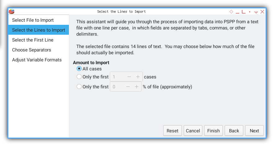
This part, I choose the second line.
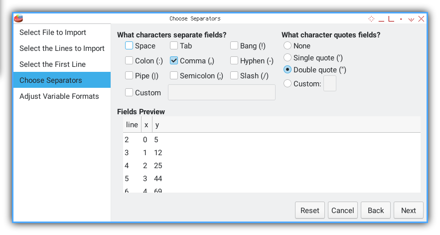
Separator.
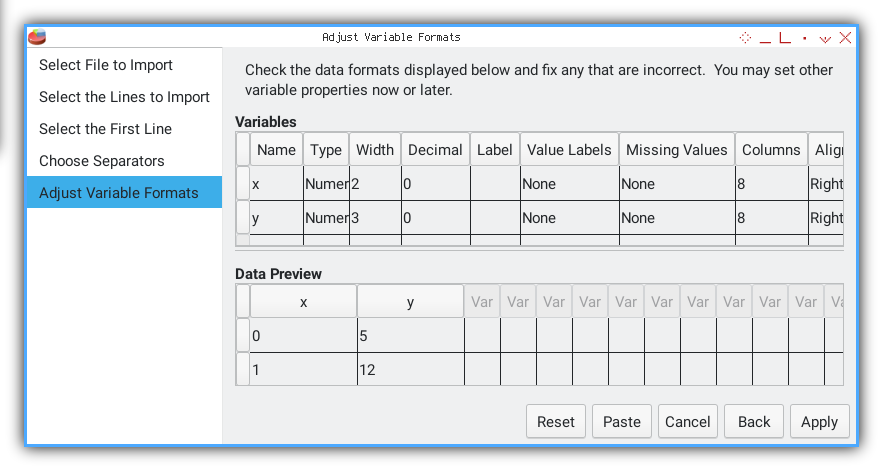
Variable format.
And you are done. You may switch to data view.
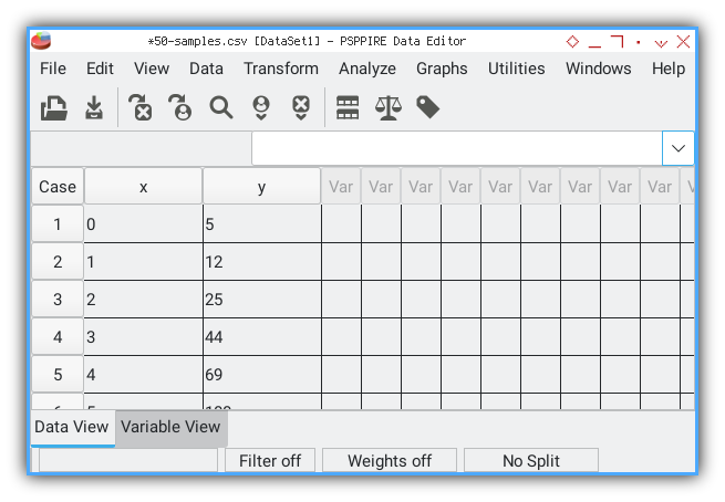
There will be other window popping up. This is the output viewer.
GET DATA
  /TYPE=TXT
  /FILE="/home/epsi/50-samples.csv"
  /ARRANGEMENT=DELIMITED
  /DELCASE=LINE
  /FIRSTCASE=2
  /DELIMITERS=","
  /VARIABLES=
    x F2.0
    y F3.0.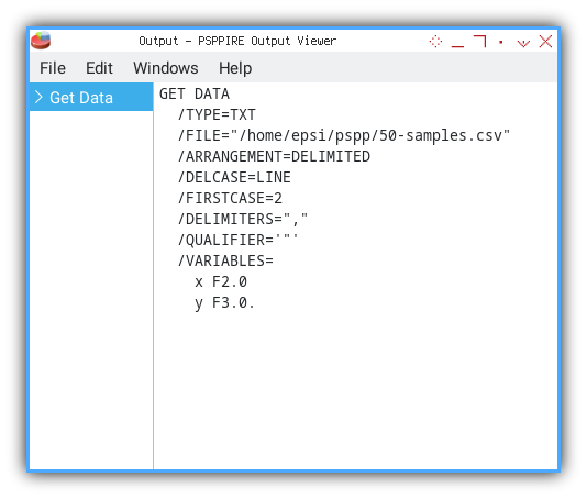
The output above is the command line.
Frequency Analysis
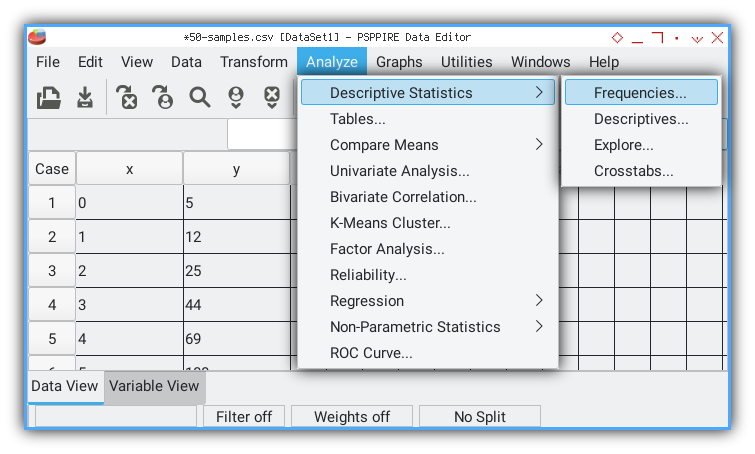
Now you can do analysis easily.
PSPPire
You can start by choosing anaylisis menu.
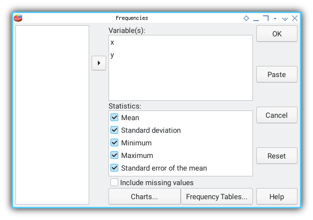
Fill the necessary dialog. Click OK.
And voila, the output viewer.
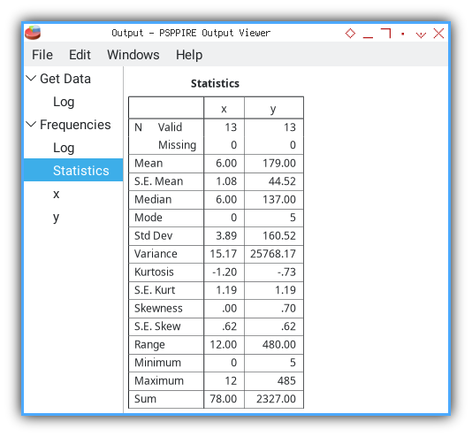
The output is similar with this below. The first text is the command line.
FREQUENCIES
	/VARIABLES= x y
	/FORMAT=AVALUE TABLE
	/STATISTICS=ALL.
Followed by tabular data of statistical properties.
        Statistics
╭─────────┬─────┬────────╮
│         │  x  │    y   │
├─────────┼─────┼────────┤
│N Valid  │   13│      13│
│  Missing│    0│       0│
├─────────┼─────┼────────┤
│Mean     │ 6.00│  179.00│
├─────────┼─────┼────────┤
│S.E. Mean│ 1.08│   44.52│
├─────────┼─────┼────────┤
│Median   │ 6.00│  137.00│
├─────────┼─────┼────────┤
│Mode     │    0│       5│
├─────────┼─────┼────────┤
│Std Dev  │ 3.89│  160.52│
├─────────┼─────┼────────┤
│Variance │15.17│25768.17│
├─────────┼─────┼────────┤
│Kurtosis │-1.20│    -.73│
├─────────┼─────┼────────┤
│S.E. Kurt│ 1.19│    1.19│
├─────────┼─────┼────────┤
│Skewness │  .00│     .70│
├─────────┼─────┼────────┤
│S.E. Skew│  .62│     .62│
├─────────┼─────┼────────┤
│Range    │12.00│  480.00│
├─────────┼─────┼────────┤
│Minimum  │    0│       5│
├─────────┼─────┼────────┤
│Maximum  │   12│     485│
├─────────┼─────┼────────┤
│Sum      │78.00│ 2327.00│
╰─────────┴─────┴────────╯
Verify Excel
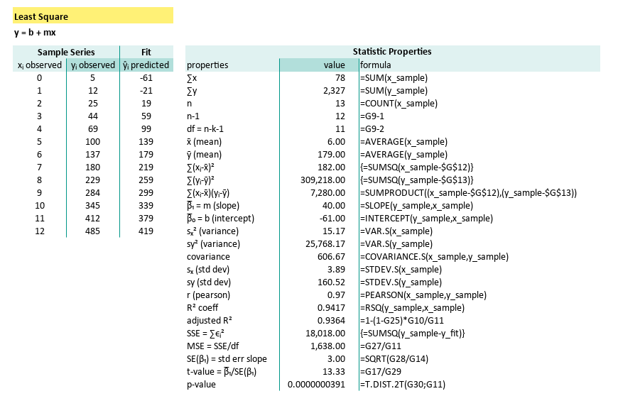
You may compare the result, with our previous calculation with Excel.
Verify Python
You may compare the result, with our previous calculation with Python.
x (max, min, range) = (   0.00,   12.00,   12.00 )
y (max, min, range) = (   5.00,  485.00,  480.00 )

x median       =      6.00
y median       =    137.00
x mode         =      0.00
y mode         =      5.00

x kurtosis     =     -1.20
y kurtosis     =     -0.73
x skewness     =      0.00
y skewness     =      0.70

x SE kurtosis  =      1.19
y SE kurtosis  =      1.19
x SE skewness  =      0.62
y SE skewness  =      0.62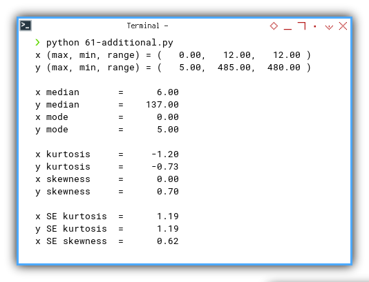
Linear Regression Analysis
You can also analyse linear regression.
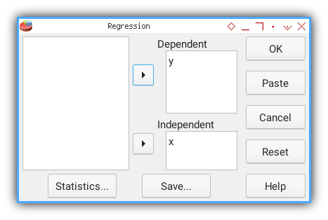
PSPPire
Again, fill the necessary dialog. Click OK.
And again, voila, the output viewer.
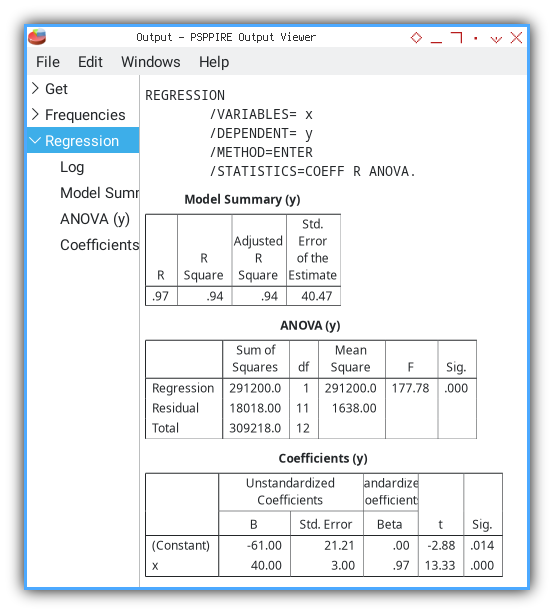
The output is similar following text. The first text is the command line. Followed by tabular data.
REGRESSION
	/VARIABLES= x
	/DEPENDENT= y
	/METHOD=ENTER
	/STATISTICS=COEFF R ANOVA.
The first is model summary. You can see the table match our previous calculation.
                     Model Summary (y)
╭───┬────────┬─────────────────┬──────────────────────────╮
│ R │R Square│Adjusted R Square│Std. Error of the Estimate│
├───┼────────┼─────────────────┼──────────────────────────┤
│.97│     .94│              .94│                     40.47│
╰───┴────────┴─────────────────┴──────────────────────────╯
The second is ANOVA. You can see the table match our previous calculation. With additional F-statistics.
                       ANOVA (y)
╭──────────┬──────────────┬──┬───────────┬──────┬────╮
│          │Sum of Squares│df│Mean Square│   F  │Sig.│
├──────────┼──────────────┼──┼───────────┼──────┼────┤
│Regression│      291200.0│ 1│   291200.0│177.78│.000│
│Residual  │      18018.00│11│    1638.00│      │    │
│Total     │      309218.0│12│           │      │    │
╰──────────┴──────────────┴──┴───────────┴──────┴────╯
The last is Coefficients. This is also match our calculation. Except that we haven’t calculate the standard error of constant yet.
                               Coefficients (y)
╭──────────┬────────────────────────────┬─────────────────────────┬─────┬────╮
│          │ Unstandardized Coefficients│Standardized Coefficients│     │    │
│          ├────────────┬───────────────┼─────────────────────────┤     │    │
│          │      B     │   Std. Error  │           Beta          │  t  │Sig.│
├──────────┼────────────┼───────────────┼─────────────────────────┼─────┼────┤
│(Constant)│      -61.00│          21.21│                      .00│-2.88│.014│
│x         │       40.00│           3.00│                      .97│13.33│.000│
╰──────────┴────────────┴───────────────┴─────────────────────────┴─────┴────╯
Verify Excel
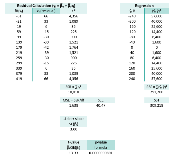
You may compare the result, with our previous calculation with excel and python.
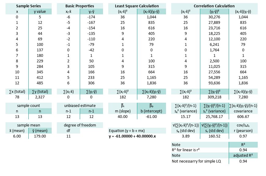
And also the right part of the worksheet.
Verify Python
You may compare the result, with our previous calculation with Python.
n          =   13
∑x (total) =   78.00
∑y (total) = 2327.00
x̄ (mean)   =    6.00
ȳ (mean)   =  179.00

∑(xᵢ-x̄)    =      0.00
∑(yᵢ-ȳ)    =      0.00
∑(xᵢ-x̄)²   =    182.00
∑(yᵢ-ȳ)²   = 309218.00
∑(xᵢ-x̄)(yᵢ-ȳ)  =   7280.00
m (slope)      =     40.00
b (intercept)  =    -61.00

Equation     y = -61.00 + 40.00.x

sₓ² (variance) =     14.00
sy² (variance) =  23786.00
covariance     =    560.00
sₓ (std dev)   =      3.74
sy (std dev)   =    154.23
r (pearson)    =      0.97
R²             =      0.94

SSR = ∑ϵ²           =  18018.00
MSE = ∑ϵ²/(n-2)     =   1638.00
SE(β₁)  = √(MSE/sₓ) =      3.00
t-value = β̅₁/SE(β₁) =     13.33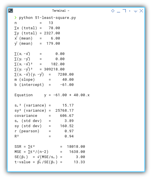
Further Analysis
If you work regularly with statistic, PSPP is your friend. There are a lot that can be done with PSPPire, but this is article is never meant to cover all PSPP feature.
I think that’s all with PSPPire.
What’s the Next Chapter 🤔?
Beside python there is this R, Julia for statistical analysis. And also Go, so you can integrate with your application seamlessly.
Consider continuing your exploration with [ Trend - Language - R - Part One ].
What’s left behind 🤔?
We are going to calculate regression for quadratic, cubic, and even spline. After that we are going to calculate correlation between two data series, with the same x-axis. Then correlation of fluctuation of, a data series against other fluctuation.