Preface
Goal: Getting to know statistical properties, using worksheet formula step by step.
When we look at regression equations in textbooks, it can feel like walking into a math dungeon without a torch. But don’t worry, we’re bringing the flashlight and a map. In this article, we’ll take the scary symbols and turn them, into something we can click and calculate in Excel. Or maybe someday Google Sheets if I, the author, have time to learn.
We’ll start with manual calculations, because understanding why something works, makes us smarter than just knowing that it works. Then we’ll show how to use built-in worksheet functions which feel like finding out, that we didn’t need to count rice grains by hand after all.
Anyone can click buttons. But knowing the guts of the formula helps us catch errors, explain our results, and feel smarter at dinner parties (or Zoom meetings).
Complete Worksheet
Yes, it looks long. Yes, it has lots of rows. But once we walk through it section by section, we will see that it is well organized. And don’t let the visual complexity fool you, this monster includes regression and correlation analysis. Two for the price of one!
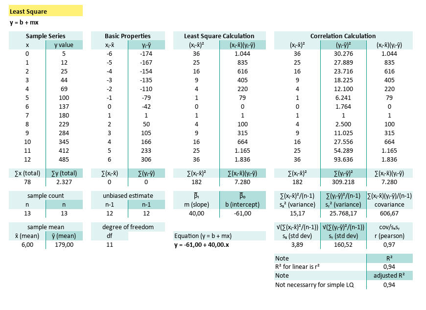
This article starting with manual calculation using Excel cells. After this section, we will reveal the built-in formulas that do all this faster.
Worksheet Source
Playsheet Artefact
You don’t have to build this from scratch (unless you’re into that). Grab the actual Excel file and tweak, break, and experiment to your heart’s content.
Known Values from Samples
Example Time! Let’s make those numbers sweat.
Imagine we’re handed a list of data points. Just plain (x, y) pairs. We don’t know where they came from, but they’re ours now, and they need analysis.
Suppose our x_observed-series lives in B7:B19,
and our y_observed-series in C7:C19.
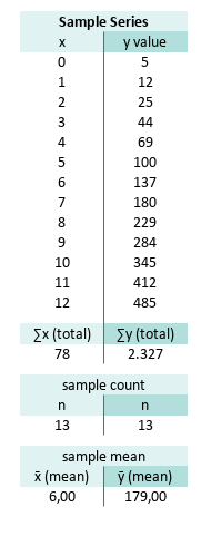
Here’s what we’re working with:
(x, y) = [(0, 5), (1, 12), (2, 25), (3, 44), (4, 69), (5, 100), (6, 137), (7, 180), (8, 229), (9, 284), (10, 345), (11, 412), (12, 485)]
We start with the basics: the mean. It is crucial for measuring how much each value wanders off.
You can calculate these with Excel’s humble built-ins:
count, sum, and average.
B22=SUM(B7:B19)
C22=SUM(C7:C19)

B26=COUNT(B7:B19)
C26=COUNT(C7:C19)

B30=AVERAGE(B7:B19)
C30=AVERAGE(C7:C19)
Or go DIY and divide the total using the sum and the count.
B30=B22/B26
C30=C22/C26
The result of the statistic properties, total and mean are:
These means will serve as the anchors for every calculation that follows. Like a good coffee shop, everything starts here.
Plot Result
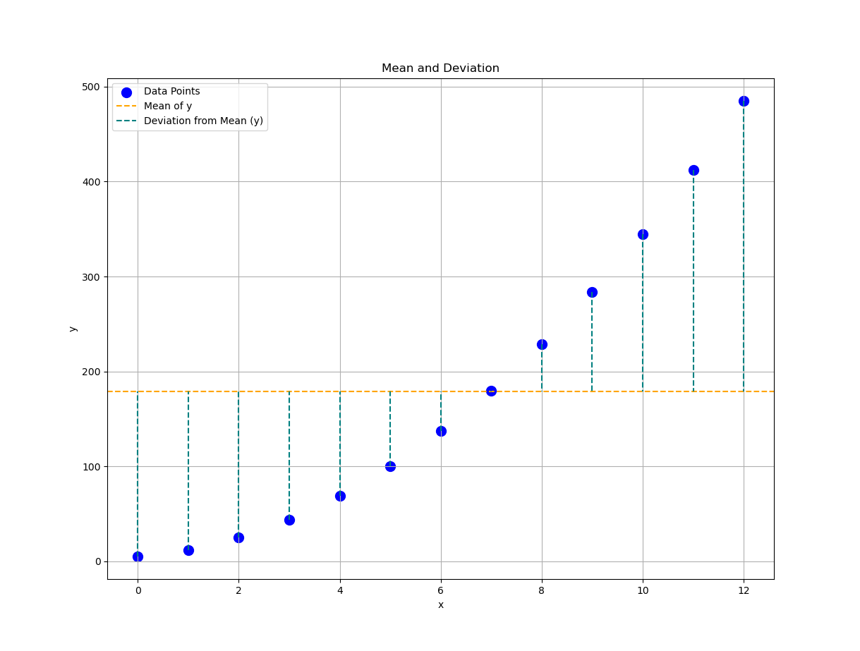
📈 Time to chart it!
Plotting these values helps us see the story our data wants to tell, before we bury it in math. Let’s see how a visualization interpret the mean properties.
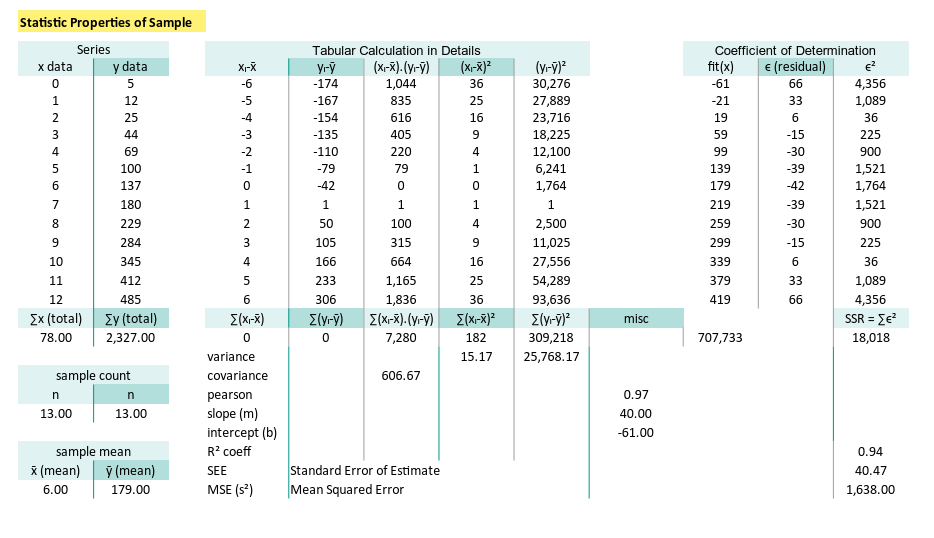
Basic Statistic Properties
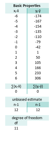
Now we can subtract, square, and stare at variances like true statisticians.
Let’s calculate how far each x_observed and y_observed,
deviate from their respective means.
This gives us the foundational ingredients for:
variance, covariance, and other buzzwords in further calculation.
For the series range E7:E19 and F7:F19 the formula are:
E7=B7-$B$30
F7=C7-$C$30
...
E19=B19-$B$30
F19=C19-$C$30
Deviations measure “how far off”, each point is from average behavior. We also need to know how many values we have, and adjust for sample size (hello, degrees of freedom).
For samples, the unbiased estimate is (n-1). I’m just following the convention to use (n-1). The math behind is a hard topic, and beyond my knowledge, so I refused to explain.
We’re not quite using df (degrees of freedom) yet, but here’s the teaser:
Translated to Excel/Calc, we can write this as:
E26=COUNT(B7:B19)-1
F26=COUNT(C7:C19)-1
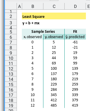
E30=COUNT(B7:B19)-2Least Square Calculation
Let’s regress it
We now compute the least squares regression, which is just a fancy way of drawing the best straight line, through our cloud of data points.
We have discuss in depth about the math behind in previous article.
The slope m (from the “famous” line equation y = mx + b) is defined as:
What we need is to find each total these properties:
- (xᵢ-x̄)²: how scattered x-values are
- (xᵢ-x̄)(yᵢ-ȳ): how x and y vary together
We need to find the nominator and the denominator.
For the series range H7:H19 (xᵢ-x̄)² and I7:I19 (xᵢ-x̄)(yᵢ-ȳ) the formula are:
H7=E7^2
I7=E7*F7
...
H19=E19^2
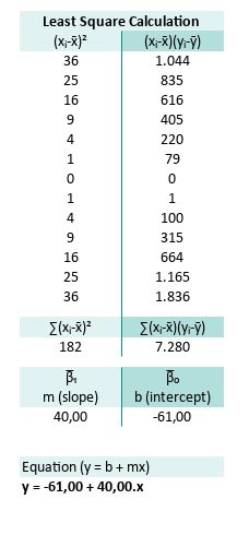
I19=E19*F19The total ∑(xᵢ-x̄)² and ∑(xᵢ-x̄)(yᵢ-ȳ) can be defined as:
H22=SUM(H7:H19)
I22=SUM(I7:I19)
The result of the each total are:
Now we got the m (slope) and b (intercept) as:
H26=I22/H22
I26=C30-H26*B30
Which gives us:
Finally we can get the full regression equation (y = b + mx) as:
H30=CONCATENATE("y = ";TEXT(I26;"#.##0,00");" + ";TEXT(H26;"#.##0,00");".x")Let’s write it in human form:
This formula gives us a predictive model.
Turn any x into an estimated y.
It’s like statistical fortune telling,
except with math instead of incense.
Again, we can see how easy it is to write down the equation in tabular spreadsheet form.
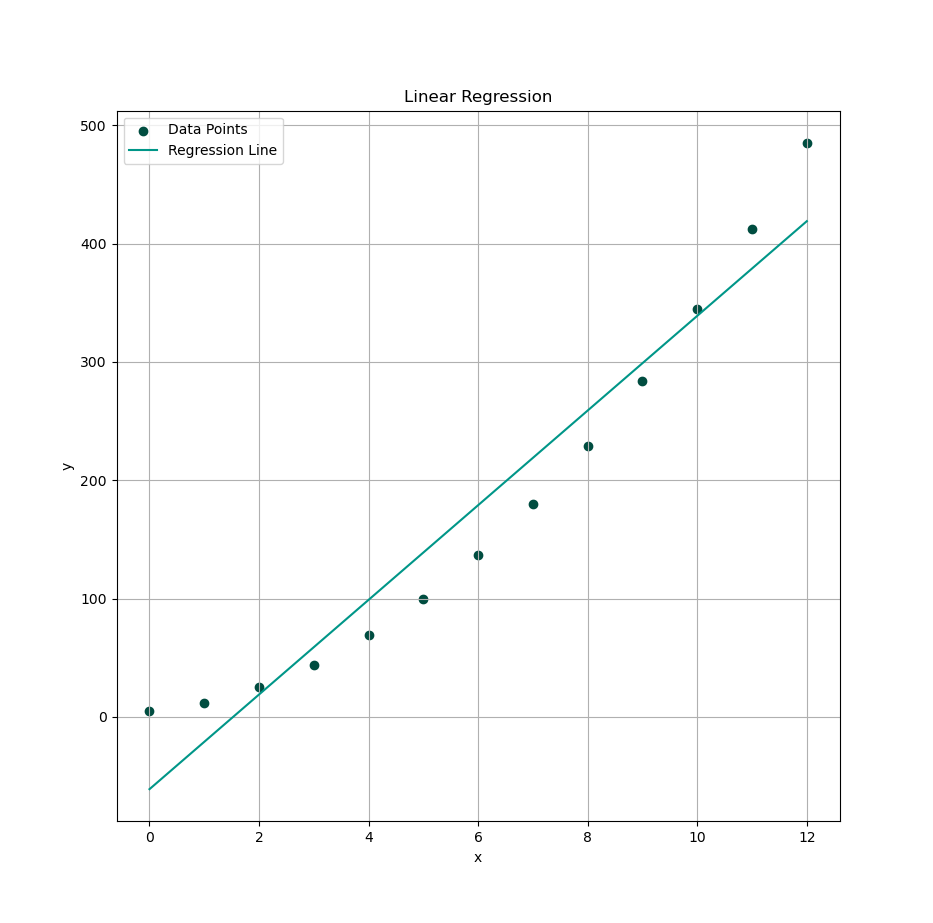
Plot Result
Time to visualize your best-fit line. Now we will see how well our equation hugs the data.
Variance and Covariance
Let’s now wander into the realm of statistical relationships, where variables whisper secrets to each other via variance and covariance. These aren’t just fancy words to impress our dinner guests, they quantify how our data behaves around its mean, and how two variables dance together.
The equations for sample variance and covariance,
for a sample of data series (x, y) is given as follows:
We’re calculating these to understand:
- (xᵢ-x̄)² and (yᵢ-ȳ)²: How much variation each variable carries
- (xᵢ-x̄)(yᵢ-ȳ): Whether the variables move together or not
For the series range K7:K19 (xᵢ-x̄)², L7:L19 (yᵢ-ȳ)²
and M7:M19 (xᵢ-x̄)(yᵢ-ȳ) the formula are:
K7=E7^2
L7=F7^2
M7=E7*F7
...
K19=E19^2
L19=F19^2
M19=E19*F19
This prepares our data for calculating how “spread out” the data is,
and whether x and y have any statistical chemistry.
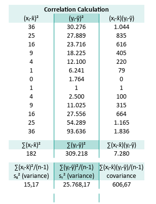
Now for the totals:
The total variation of the predictor, ∑(xᵢ-x̄)², (yᵢ-ȳ)² and ∑(xᵢ-x̄)(yᵢ-ȳ) can be defined as:
K22=SUM(K7:K19)
L22=SUM(L7:L19)
M22=SUM(M7:M19)
The result of the each total are:
To normalize these (and avoid bias ) we divide by degrees of freedom (n - 1). Now we got the variance sₓ², sy² and also the covariance as:
K22=K22/E26
L22=L22/F26
M22=M22/E26
The result of the statistic properties are:
Variance tells us how unpredictable the data is, and covariance gives us a sneak peek into, whether the two variables move together (positive), apart (negative), or ignore each other entirely (zero, the statistical equivalent of ghosting).
The tabular spreadsheet can be shown as follows:
Oh, and standard deviation is just the square root of variance.
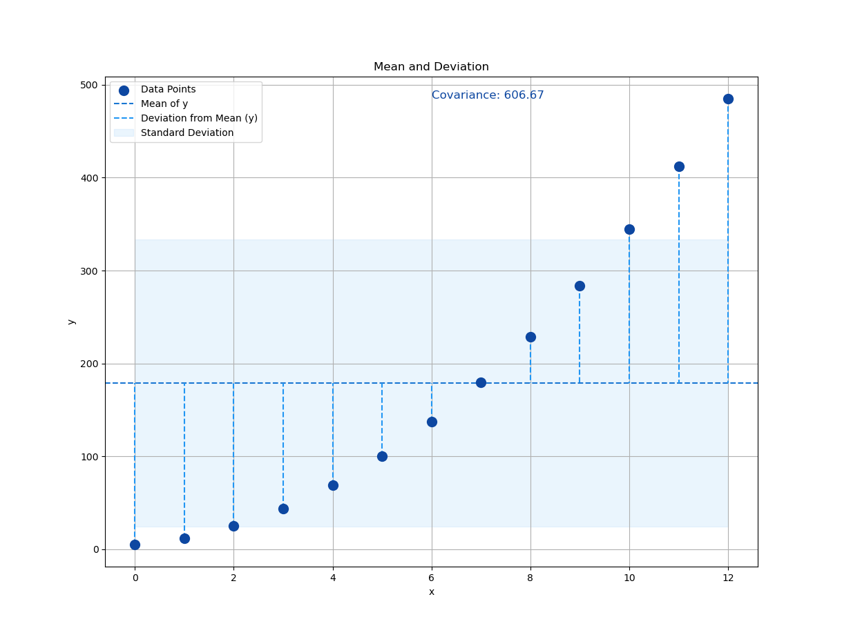
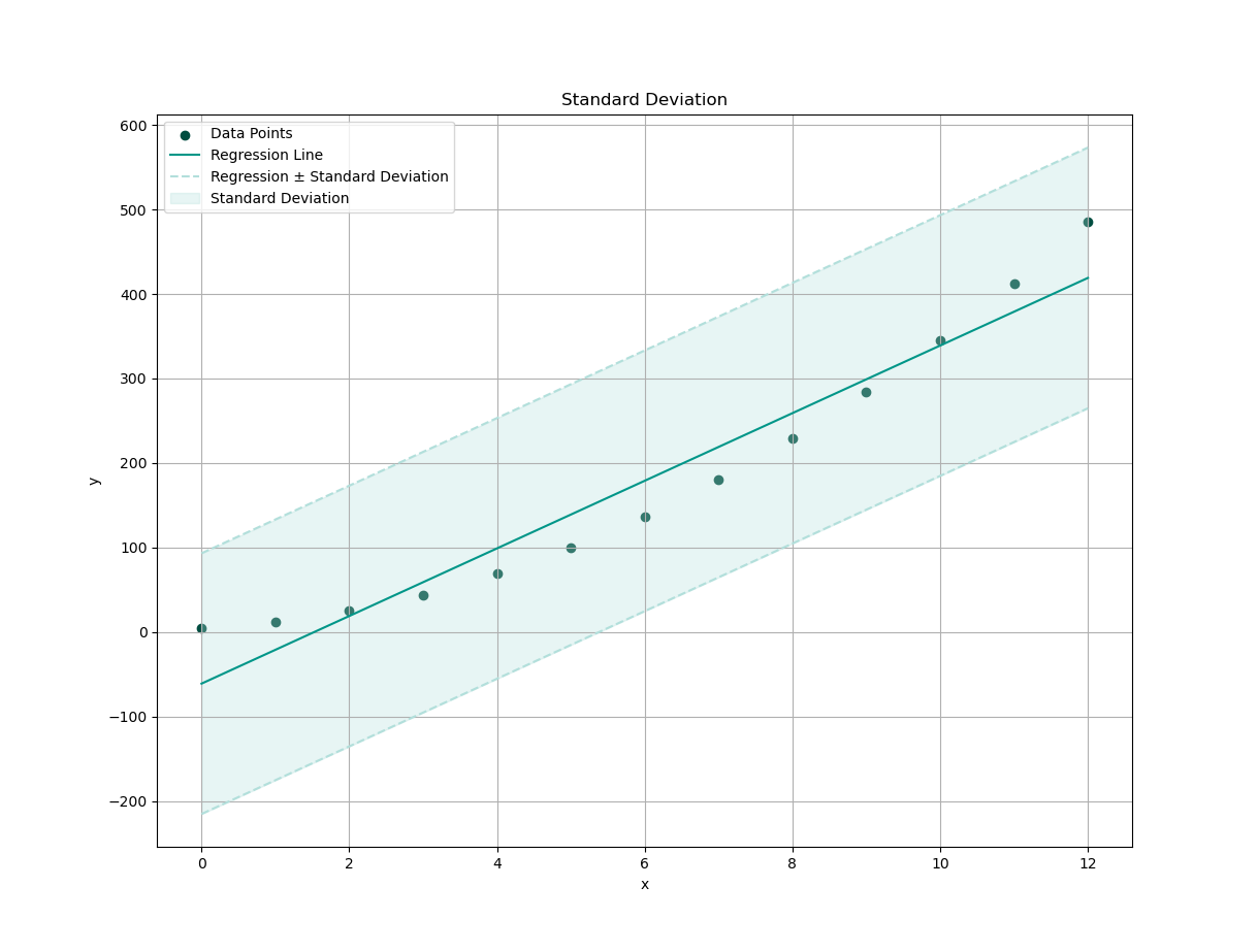
Plot Result
We need a visualization so we can interpret the standard deviation properties against original observed y.
Correlation Calculation
Time to put the cool shades on our statistics. Let’s measure correlation, the standardized version of covariance, that fits nicely between -1 and 1.
From calculated properties above we can continue to standard deviation sₓ, sy, along with the r (pearson) value:
K30=SQRT(K26)
L30=SQRT(L26)
M30=M26/(K30*L30)
This yields:
A correlation coefficient of 0.97? That’s about as close to a linear relationship as you can get, without your data actually proposing marriage.
Note that the pearson coefficient can be denoted in different form. Alternative formula for r (same dance, different choreography):
r = cov/sₓsy
r = (∑(xᵢ-x̄).(yᵢ-ȳ))/√(∑(xᵢ-x̄)².∑(yᵢ-ȳ)²)
This way we can calculate the R square (R²) and also the adjusted R square. Note that R² for simple linear sample is the same as r². In this case R² = 0,9417. But the R² might be different for complex cases.
M33=M30^2Also there is no need any adjusted R², for simple least square population. But for sample we need to adjust with k=1, for linear equation then adjusted R² = 0,9364.
M35=1-(1-M33)*(B26-1)/(B26-1-1)We can have a look at the result, focusing on this part of following spreadsheet:
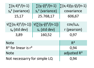
R² = 0.94 → “94% of the variance in y is explained by x.”
That’s nearly everything, the other 6% probably noise,
or maybe just forgot to update their spreadsheets.
Plot Result
We need a visualization so we can interpret the standard deviation properties against predicted y.
Residual Calculation
Finally, we measure how far off our predictions are. Every prediction has regrets, and in statistics, they’re called residuals.
We plug in our linear model from the coefficient of the linear least square,
- m (slope)
- b (intercept)
We can built our curve fitting equation (y = b + mx), and predict every yᵢ value.
Use the spreadsheet to compute.
For the series range O7:O19 fit(xᵢ), P7:P19 ϵᵢ (residual),
and Q7:Q19 ϵᵢ² the formula are:
O7=$I$26+$H$26*B7
P7=C7-O7
M7=P7^2
...
O19=$I$26+$H$26*B19
P19=C19-O19
M19=P19^2
Note that we can use any curve fitting formula, such as quadratic, cubic and so on, but for this example we will use our linear one.
Now total residual error. The total of ϵᵢ² can be defined as:
Q22=SUM(Q7:Q19)The result of the each total are:
The tabular spreadsheet can be shown as follows:
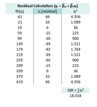
Residuals show us where our model is off. If the residuals are too wild, the model might just be blowing statistical smoke.
Plot Result
We need a plot to show,
how far off the actual y_predicted is,
from our model’s predictions.
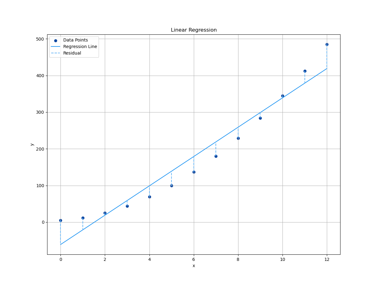
Plotting residuals is like proofreading our math. Weou don’t always like what we see, but it makes everything better.
Regressions Sum Square
Welcome to the world of SSR, Regression Sum of Squares, or as we statisticians like to call it: “How much our predictions flex on the average.” Here is the RSS:
This represents the variation explained by our model. The bigger it is (relative to total variance), the more our model is saying, “Hey, I actually know what’s going on!”
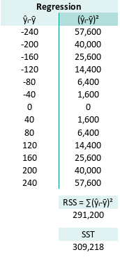
Naturally, this brings us to SST. Sum of Squares Total, a.k.a. the full buffet of variance:
The SST (Sum Square Total) is
Mathematically, for each observed yᵢ, we can say:
Yes, it’s a love triangle. The total variation (SST) is shared between,
- what the model explains (RSS, Regressions Sum Square) and,
- what it misses (SSR, Sum of Squares of Residual).
Why does SST = SSR + RSS?
It is easier to understand using the spreadsheet.
This equation is rooted in partitioning variance. Essentially slicing up the total variation in our data into:
-
RSS = Regression Sum of Squares (explained): The variation due to the model. It’s how much our predicted values
ŷᵢ deviate from the meanȳᵢ. If this is large, our model is picking up real structure in the data. -
SSR = Sum of Squares of Residual (unexplained): What’s left over, the part of the variance our model fails to explain, .e., the noisy, chaotic behavior of real-world data. It is how far off our predictions are from the actual
yᵢvalues. Ideally, this is small. -
SST = Total Sum of Squares: The total variation in the dependent variable
yᵢ. essentially: “How spread out is y overall, around its mean?”
Our model projects the data onto a line, and splits perfectly between “explained” and “unexplained.”
Back to R²
This is the statistical backbone of R². Want to know how good our regression line is? Start here. It’s the source of model validation.
R² (coefficient of determination) is defined as:
It answers, “How much of the variation in y is captured by x?”
-
If R² = 1, our model explains everything. Congratulations, we’ve either modeled reality perfectly, or we’ve committed statistical heresy (i.e., overfitting).
-
If R² = 0, our model explains nothing, It’s as useful as a horoscope.
t-value and p-value
Truth or Dare?
Now for the dramatic part, the hypothesis testing,
using t-value and p-value.
We want to know: “Is our slope real or just a fluke?”
First, calculate the degrees of freedom,
For linear equation k=1.
In Excel/Calc we can write this as:
E30=COUNT(B7:B19)-2Degrees of freedom are like free will in data. The more we have, the more trust we can put in our analysis.
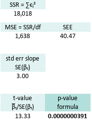
Next, enter the Mean Squared Error. It tells us how wrong the model is, on average, for each point:
In Excel/Calc we can write this as:
=Q22/$E$30Then we compute the Standard Error of the Slope SE(β1) using MSE.
In Excel/Calc we can write this as:
=SQRT(Q25/K22)Next, the t-value: This is where we look slope in the eye,
and say: “Prove you matter.”
The t-value for the slope coefficient (β₁) is computed,
as the ratio of the estimated slope (βˉ₁),
to the standard error of the slope (SE(β₁)).
This t-value will be used to test the null hypothesis,
that the true slope coefficient is equal to zero.
In Excel/Calc we can write this as:
=H26/Q30And finally, the p-value, the real drama queen.
It’s the probability that our slope is due to random chance.
The smaller the p-vlue, the more confident we are,
that our model actually means something.
Here is the p-value for two tail test.
This is to complex for manual calculation. so I use built-in formula instead.
In spreadsheet speak:
=T.DIST.2T(Q35;$E$30)The p-value is our model’s confession.
It either says: “"Yep, I’m legit,”,
or “Oops, maybe I was just noise.”
Here are the results of this statistical soap opera:
We have an incredibly significant result. Oour slope isn’t just a good guess, it’s a statistically valid superstar.
Check it out here:
We have a good confidence in our curve fitting function.
Alternative Worksheet
If you'‘e not into one worksheet layout, don’t worry. Spreadsheet is like statistics: it tolerates many truths.
Here’s an alternative way of laying things out:
Just remember, the numbers must dance the same. No matter how we rearrange the ballroom.
Built In Formula
The Lazy Genius of Regression
Who needs to crunch numbers by hand, when spreadsheets and Python will gladly do our bidding? Let’s explore how built-in formulas make regression analysis, feel less like statistical calculus, and more like statistical calculus-on-autopilot.
Worksheet Source
Your DIY Regression Playground
Welcome to spreadsheet heaven.
You’ll find all the formulas preloaded in this .ods file.
Even though everything here can work in Excel,
we’re using LibreOffice.
Why? Because .ods lets us play with named ranges more flexibly,
and frankly, .xlsx sometimes throws a tantrum.
Still prefer Excel? We got you:
Meet the Data
Let’s revisit our familiar cast of statistical characters:
- xᵢ observed:
B7:B19, - yᵢ observed:
C7:C19, - ŷᵢ predicted:
D7:D19calculated from m and b.
Named Range
B7:B19 is Not a Personality
To make the equation less cryptic, we can define named range. This can be done in both Excel and Calc:
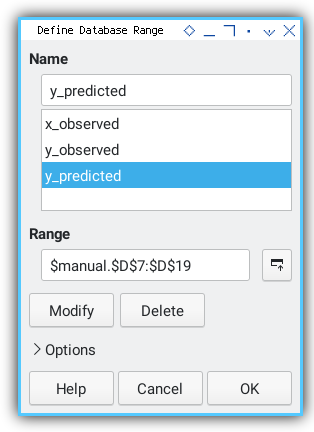
Let’s give our ranges real names. “x_observed” just sounds more mature than “B7:B19”.
B7:B19: x_observed.C7:C19: y_observed.D7:D19: y_predicted.
Think of it as giving our variables, name tags at a regression conference.
Using Array Operation
We can rebuild tabular woksheet from previous article,
into a simple one using Excel/Calc formula
with the help of SUMSQ formula.
With just using array formulas and built-in functions, we can have direct result into a cell. Because if Excel has a button for it, why type three columns by hand?
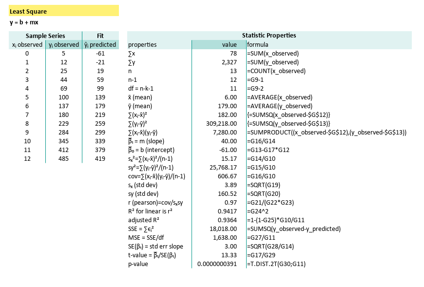
Here the predicted value of ŷᵢ in D7:D19,
are calculated from m ($G$17) and b ($G$18).
The complete formula can be shown here:
| properties | formula |
|---|---|
| ∑x | =SUM(x_observed) |
| ∑y | =SUM(y_observed) |
| n | =COUNT(x_observed) |
| n-1 | =G9-1 |
| df = n-k-1 | =G9-2 |
| x̄ (mean) | =AVERAGE(x_observed) |
| ȳ (mean) | =AVERAGE(y_observed) |
| ∑(xᵢ-x̄)² | {=SUMSQ(x_observed-$G$12)} |
| ∑(yᵢ-ȳ)² | {=SUMSQ(y_observed-$G$13)} |
| ∑(xᵢ-x̄)(yᵢ-ȳ) | =SUMPRODUCT((x_observed-$G$12),(y_observed-$G$13)) |
| β̅₁ = m (slope) | =G16/G14 |
| β̅₀ = b (intercept) | =G13-G17*G12 |
| sₓ²=∑(xᵢ-x̄)²/(n-1) | =G14/G10 |
| sy²=∑(yᵢ-ȳ)²/(n-1) | =G15/G10 |
| cov=∑(xᵢ-x̄)(yᵢ-ȳ)/(n-1) | =G16/G10 |
| sₓ (std dev) | =SQRT(G19) |
| sy (std dev) | =SQRT(G20) |
| r (pearson)=cov/sₓsy | =G21/(G22*G23) |
| R² for linear is r² | =G24^2 |
| adjusted R² | =1-(1-G25)*G10/G11 |
| SSE = ∑ϵᵢ² | {=SUMSQ(y_observed-D7:D19)} |
| MSE = SSE/df | =G27/G11 |
| SE(β₁) = std err slope | =SQRT(G28/G14) |
| t-value = β̅₁/SE(β₁) | =G17/G29 |
| p-value | =T.DIST.2T(G30;G11) |
We’re covering all our greatest statistical hits: slope, variance, correlation, R², t-tests, and the always-glamorous p-value.
This condenses a ton of regression math, into digestible spreadsheet logic. Less time formatting cells, more time eating snacks and doing science.
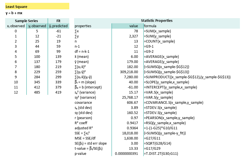
Using Statistic Formula
The Built-in Shortcut
Furthermore we can use statistic formula.
Want to double-check your math? Or just feel like living dangerously by trusting Excel’s statistical engine? Let’s name new ranges for a fresh worksheet:
B7:B19: x_sample.C7:C19: y_sample.D7:D19: y_fit.
Then we let built-in stats formulas take over.
| properties | formula |
|---|---|
| ∑x | =SUM(x_sample) |
| ∑y | =SUM(y_sample) |
| n | =COUNT(x_sample) |
| n-1 | =G9-1 |
| df = n-k-1 | =G9-2 |
| x̄ (mean) | =AVERAGE(x_sample) |
| ȳ (mean) | =AVERAGE(y_sample) |
| ∑(xᵢ-x̄)² | {=SUMSQ(x_sample-$G$12)} |
| ∑(yᵢ-ȳ)² | {=SUMSQ(y_sample-$G$13)} |
| ∑(xᵢ-x̄)(yᵢ-ȳ) | =SUMPRODUCT((x_sample-$G$12),(y_sample-$G$13)) |
| β̅₁ = m (slope) | =SLOPE(y_sample,x_sample) |
| β̅₀ = b (intercept) | =INTERCEPT(y_sample,x_sample) |
| sₓ² (variance) | =VAR.S(x_sample) |
| sy² (variance) | =VAR.S(y_sample) |
| covariance | =COVARIANCE.S(x_sample,y_sample) |
| sₓ (std dev) | =STDEV.S(x_sample) |
| sy (std dev) | =STDEV.S(y_sample) |
| r (pearson) | =PEARSON(x_sample,y_sample) |
| R² coeff | =RSQ(y_sample,x_sample) |
| adjusted R² | =1-(1-G25)*G10/G11 |
| SSE = ∑ϵᵢ² | {=SUMSQ(y_sample-y_fit)} |
| MSE = SSE/df | =G27/G11 |
| SE(β₁) = std err slope | =SQRT(G28/G14) |
| t-value = β̅₁/SE(β₁) | =G17/G29 |
| p-value | =T.DIST.2T(G30;G11) |
The parameter required for each statistic formula is clear now. These functions reduce error and save time. Perfect when we’ve had our third coffee, and still can’t remember what ∑(xᵢ - x̄)² stands for.
Pearson Correlation Coeffecient
Measuring Statistical Chemistry
Need to measure the linear love between x and y?
Use Pearson’s r correlation coefficient:
=PEARSON(B7:B19;C7:C19) The formula for pearson is:
Which we can write manually in Excel/Calc as:
=COVARIANCE.P(B7:B19, C7:C19) / (STDEV.P(B7:B19) * STDEV.P(C7:C19))And if you’re feeling masochistic, the Pearson correlation coefficient can also be expressed as follows:
Sometimes you want to check if your equation right. Again, the Excel/Calc formula can be rewritten as follows, and having the same result.
= (SUM((B7:B19 - AVERAGE(B7:B19)) * (C7:C19 - AVERAGE(C7:C19))))
/ (SQRT(SUM((B7:B19 - AVERAGE(B7:B19))^2) * SUM((C7:C19 - AVERAGE(C7:C19))^2)))
Now you know, how helpful the built-in formula is, compared to this complex formula above.
R Square
The MVP of Model Metrics
Want to know how much of the variation in y is explained by our model?
Excel/Calc has a built-in formula for R Square (R²):
=RSQ(C7:C19;B7:B19)The R Square (R²) for simple linear regression can be expressed as follows:
Here’s the long-form version. The general R Square (R²) is defined as:
Or furthermore, we can go low-level.
Down to the nuts and bolts, the Excel/Calc formula can be rewritten as:
=1-SUM((C7:C19 - (B7:B19*G22+G24))^2)/SUM((C7:C19 - H9)^2)The way you manage the calculation is depend on your situation.
Most of the time we can use simple rsq formula,
but sometimes we need to go low level,
for use with programming or just intellectual curiosity.
Let’s see how RSQ behave in non-linear curve fitting discussed later on.
Compare and Contrast: Manual vs Built-in
Feel free to compare both methods, side-by-side. Between manual formula and built-in formula as shown below:
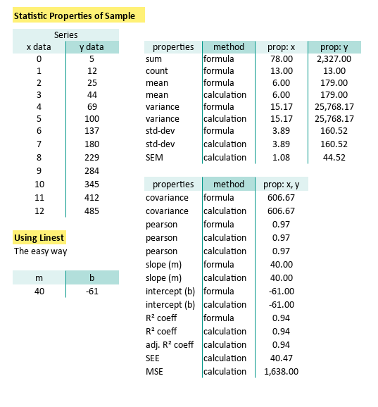
Like a true stats nerd, always double-check our work. But also, enjoy the shortcuts modern tools give us. Regression shouldn’t feel like a root canal.
Now we are ready to make statistical model, in our worksheet to suit our specific needs.
How you make the model is up to you.
What Lies Ahead 🤔?
That method above? Elegant, yes. But let’s not kid ourselves. Naturally, there’s a simpler way.
If we want a spreadsheet model that doesn’t require a PhD. Or three cups of coffee and a blank stare, we’ll need a method more fit for everyday use. Something robust, readable, and less likely to induce formula fatigue.
The easier it is to calculate, the more likely we’ll actually use it. That’s why in the next part of our adventure, we shift gears from cells and formulas, to the comforting embrace of Python. There, we’ll build tools that are both reusable, and less fiddly than spreadsheet gymnastics.
Grab our virtual lab coat and join us in: [ Trend - Properties - Python Tools ].