Trend - Polynomial Examples

Trend: Introduction

Trend: Enhanced

Trend: Language

Local Group

Preface

Goal: Curve fitting examples for daily basis, using vandermonde matrix.

For daily basis, we do not need to derive mathematical equation at all. We can utilize ready to use worksheet and python script.

I have prepared a workbook containing different worksheet:

Linear Equation (first order polynomial)
Quadratic Equation (second order polynomial)
Cubic Equation (third order polynomial)

Spreadsheet: Workbook with Multiple Worksheet

Following previous article, each case has three steps:

From the known coefficient, find the points (x, y).
Building the matrix visually, based on equation of the system.
From the points (x, y), find the coefficient. Inverse the matrix, solving the equation.

For daily basis, all you need is just the last sheet (matrix inverse) of selected case (order). The real data for daily basis is dispersed, unlike given data in this example sheet.

The worksheet is pretty explanatory. Assuming that you have read previous article, The first and the second sheet is, already well explained in previous article, so we are going to skip these sheets. I do not think that I should explain each worksheet in detail.

The python script also has been explained in previous article, the purpose of this exampale is just giving a ready to use script. So I won’t go into detail either.

Other Method

Vandermonde matrix is not the only method to get polynomial equation. We are going to use Least Square method later.

Worksheet Source

Playsheet Artefact

The Excel file is available, so you can have fun, modify as you want.

github.com/…/math/trend/examples-polynomial.xlsx

1: Linear Equation

First Order Polynomial Method

Curve Fitting

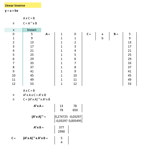
Since real data matrix is definitely not a square matrix, and matrix inverse can only work with square nxn matrix. We need to alter the equation with transpose.

$\begin{aligned} && A \times \mathbf{C} &= \mathbf{B} \\ \Rightarrow && A^T \times A \times \mathbf{C} &= A^T \times \mathbf{B} \\ \Rightarrow && \mathbf{C} &= (A^T \times A)^{-1} \times (A^T \times \mathbf{B}) \end{aligned}$

Here is the visual implementation in spreadsheet.

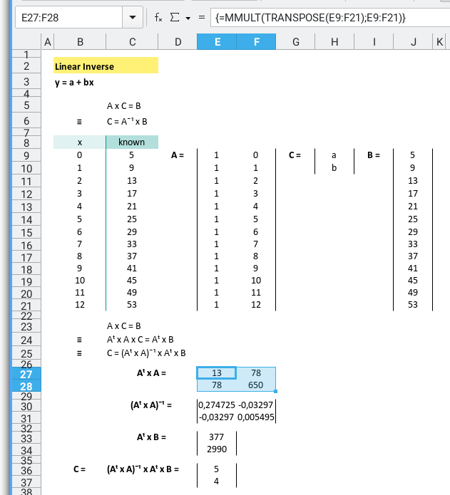
Polynomial: Worksheet: Linear Equation: Getting Coefficient

The formula in spreadsheet are as below:

$A^T \times A$

=MMULT(TRANSPOSE(E9:F21);E9:F21)

then inverse

$(A^T \times A)^{-1}$

=MINVERSE(E27:F28)

then inverse

$A^T \times \mathbf{B}$

then continue

=MMULT(TRANSPOSE(E9:F21);J9:J21)

and finally the solution

$\mathbf{C} = (A^T \times A)^{-1} \times (A^T \times \mathbf{B})$

then continue

=MMULT(E30:F31;E33:E34)

Let’s clean the spreadsheet view.

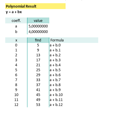
Polynomial: Worksheet: Linear Equation: Getting Coefficient

With the coefficient below:

$\begin{aligned} a &= 5 \\ b &= 4 \\ \end{aligned}$

And known x for this equation

$\begin{aligned} x_i &= [0, 1, 2, \ldots, 10, 11, 12] \\ y_i &= a + bx_i \end{aligned}$ We can calculate y` by using spreadsheet formula.

=$C$43+$C$44*B47

The prediction value can be shown as spreadsheet below:

Polynomial: Worksheet: Linear Equation: Predicting Values

Python Scripts

Instead of hardcoded data, we can setup the source data in CSV.

github.com/…/trend/31-linear-equation.csv

The CSV looks like this file below:

x,y
0,5
1,9
2,13
3,17
4,21
5,25
6,29
7,33
8,37
9,41
10,45
11,49
12,53

The python source can be obtained from below link

github.com/…/trend/31-linear-equation.py

It is very similar with source code in previous article, except that it is for linear equation. So I don’t think that I should explain into the detail.

# Initial Matrix Value
order = 1

# Getting Matrix Values
mCSV = np.genfromtxt("31-linear-equation.csv",
  skip_header=1, delimiter=",", dtype=float)

...

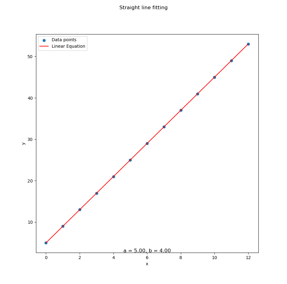
With data series in CSV above we can get all curve fitting as below:

Python: Matplotlib Result: Linear Equation

Interactive JupyterLab

You can obtain the interactive JupyterLab in this following link:

github.com/…/trend/31-linear-equation.ipynb

2: Quadratic Equation

Second Order Polynomial Method

Curve Fitting

With the same step as above linear system equation, we can get visual implementation in spreadsheet of quadratic system equation.

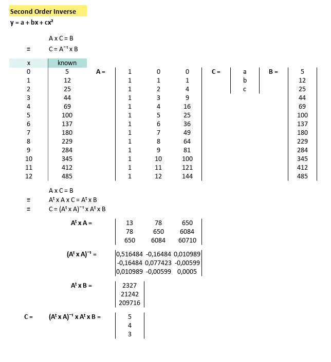
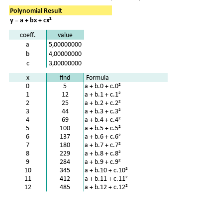
Polynomial: Worksheet: Quadratic Equation: Getting Coefficient

With can write the result as coefficient below:

$\begin{aligned} a &= 5, & b &= 4, & c &= 3 \end{aligned}$

With known x for this equation, we can calculate y by using spreadsheet formula.

$\begin{aligned} x_i &= [0, 1, 2, \ldots, 10, 11, 12] \\ y_i &= a + bx_i + cx_i^2 \end{aligned}$

The prediction value can be shown as spreadsheet below:

Polynomial: Worksheet: Quadratic Equation: Predicting Values

Python Scripts

Instead of hardcoded data, we can setup the source data in CSV.

github.com/…/trend/32-data-second-order.csv

The CSV looks like this file below:

x,y
0,5
1,12
2,25
3,44
4,69
5,100
6,137
7,180
8,229
9,284
10,345
11,412
12,485

The python source can be obtained from below link

github.com/…/trend/32-poly-second-order.py

It is very similar with source code in previous article, except that it is for quadratic equation. So again, I don’t think that I should explain into the detail.

# Initial Matrix Value
order = 2

# Getting Matrix Values
mCSV = np.genfromtxt("32-data-second-order.csv",
  skip_header=1, delimiter=",", dtype=float)

...

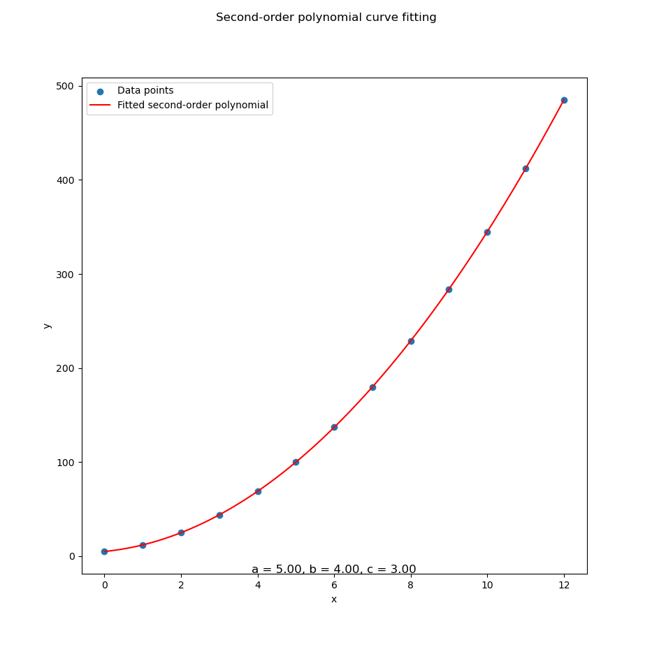
With data series in CSV above we can get all curve fitting as below:

Python: Matplotlib Result: Second Order Polynomial

Interactive JupyterLab

You can obtain the interactive JupyterLab in this following link:

github.com/…/trend/32-poly-second-order.ipynb

3: Cubic Equation

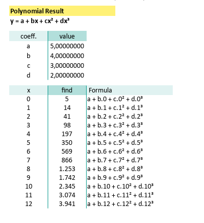
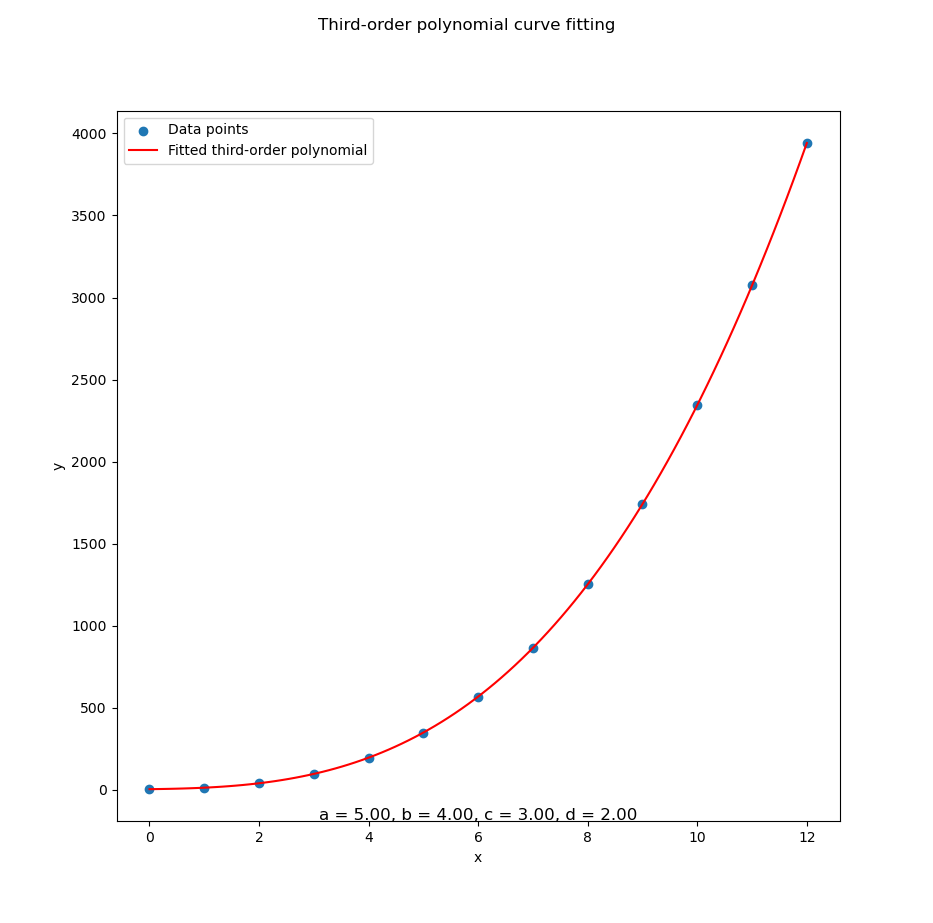
Third Order Polynomial Method

Curve Fitting

With the same step as above linear system equation, we can get visual implementation in spreadsheet of cubic system equation.

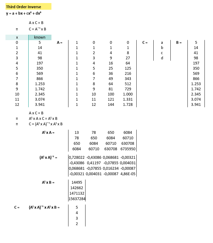
Polynomial: Worksheet: Cubic Equation: Getting Coefficient

With can write the result as coefficient below:

$\begin{aligned} a &= 5, & b &= 4, & c &= 3, & d &= 4. \end{aligned}$

With known x for this equation, we can calculate y by using spreadsheet formula.

$\begin{aligned} x_i &= [0, 1, 2, \ldots, 10, 11, 12] \\ y_i &= a + bx_i + cx_i^2 + dx_i^3 \end{aligned}$

The prediction value can be shown as spreadsheet below:

Polynomial: Worksheet: Cubic Equation: Predicting Values

Python Scripts

Instead of hardcoded data, we can setup the source data in CSV.

github.com/…/trend/33-data-third-order.csv

The CSV looks like this file below:

The python source can be obtained from below link

github.com/…/trend/33-poly-third-order.py

It is very similar with source code in previous article, except that it is for quadratic equation. So again, I don’t think that I should explain into the detail.

# Initial Matrix Value
order = 3

# Getting Matrix Values
mCSV = np.genfromtxt("33-data-third-order.csv",
  skip_header=1, delimiter=",", dtype=float)

...

With data series in CSV above we can get all curve fitting as below:

Python: Matplotlib Result: Third Order Polynomial

Interactive JupyterLab

You can obtain the interactive JupyterLab in this following link:

github.com/…/trend/33-poly-third-order.ipynb

What’s the Next Chapter 🤔?

There is also a more powerful approach to solve curve fitting. It is the least square, starting from linier, and then we can continue exploring quadratic and also cubic. This way we can step on the regression and also correlation analysis. However we should step-in from the simple thing. It is the linear least square.

Consider progressing further by exploring the next topic: [ Trend - Least Square ].