Trend - Properties - Cheatsheet

Trend: Prediction

Trend: Regression

Trend: Enhanced

Trend: Language

Local Group

Preface

Goal: Getting to know statistical properties, equation by cheatsheet step by step.

Let’s face it: when things get messy (and they will), we’ll need more than just good vibes and Google. Whether we’re double-checking a suspiciously magical result from a Python library, or debugging a spreadsheet that’s decided to betray us, manual math is our lifeline.

Sure, there are calculators online. There are tools that promise answers with zero thinking required. But here’s the catch: if we can’t follow the math, how do we know it’s not lying to us?

The Inner Working

“In regression we trust, but always verify.” 😄

So before we get cozy with automated libraries or built-in spreadsheet functions, we’ll walk through the equations. Old school. Like our stats professor, but with slightly better graphics.

Basic math is required But we don’t have to do math by hand forever, that’s what machines are for. However, we do need to understand how it works, at least once. So we can catch bugs, tweak models, and sound convincing in a meeting.

Think of this cheat sheet as our statistical Rosetta Stone: a reference to demystify the math behind linear regression.

Let’s get it on!

Cheatsheet

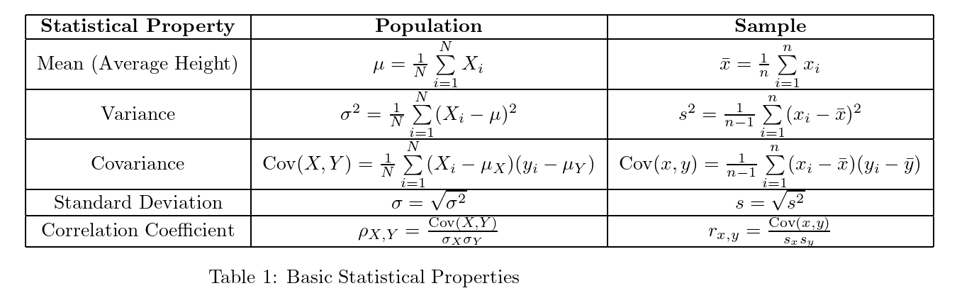
For simplicity, we’re working with sample statistics here. Note that population and samples has different notation. Population equations differ slightly (and judge us silently when we confuse them). We will deal with those later.

Here’s a high-level view of what’s involved, in a basic least squares regression:

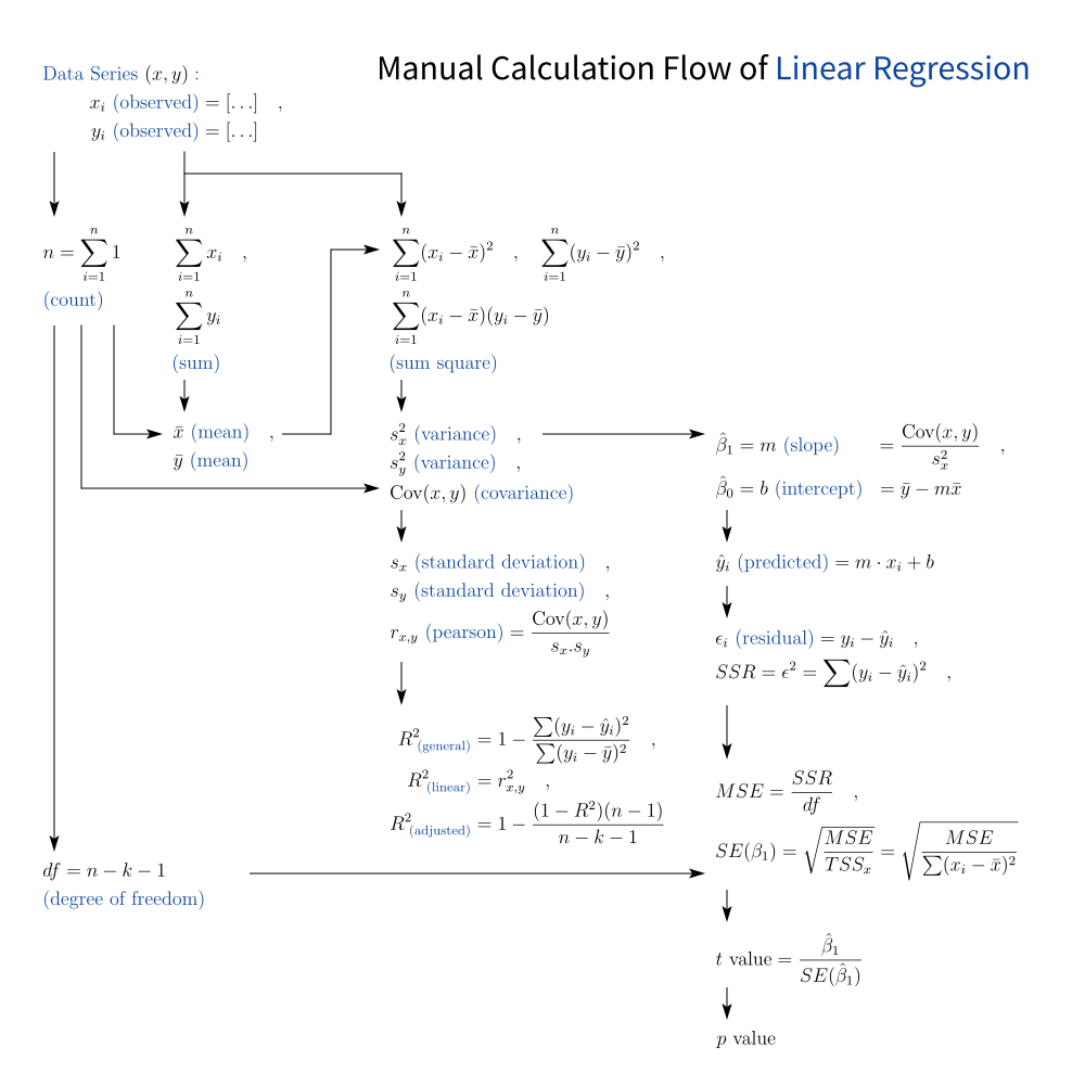
Trend: TeX: Cheatsheet: Equation Flow

Yes, it looks like the math equivalent of a subway map, but every symbol here has a job. And no, none of them are optional.

We can download and remix the full diagram:

This cheat sheet is a foundation we’ll keep returning to, especially when exploring correlation, residuals, and how to impress your data team with Greek letters.

If you disagree with my math, feel free to correct it. I welcome pull requests and polite statistical debates.

1: Equation for Linear Regression

Least Square Method

In a previous article, we dipped our toes into the least squares method. Think of it as statistics’ way of drawing the “best guess” line through a crowd of noisy data points. But regression isn’t just about drawing lines. It’s about understanding the math behind the curtain.

In this article, we’ll cover more essential statistical properties, like variance, covariance, correlation, and everyone’s favorite: R² (which sounds like a robot but is sadly less cute).

Trend: TeX: Cheatsheet: Population and Sample

You can download the full cheatsheet diagram in raw LaTeX from here:

github.com/…/math/trend/50-cheatsheet.tex

Regression analysis isn’t just a plug-and-play task. Whether we’re working in Excel or Python, these formulas help us:

Sanity-check built-in results
Understand what the software is actually calculating
Speak with authority in meetings ("Clearly, the low R² suggests heteroscedasticity.” Boom. Respect.)

Data Series

The Usual Suspects

With sample of data points

$\begin{array}{|c|c|} \hline x_i & \textbf{observed x} \\ \hline y_i & \textbf{observed y} \\ \hline \hat{y}_i & \textbf{predicted y} \\ \hline \end{array}$

These will appear in every equation. Think of them as the cast of characters in our regression drama.

Total

The count and sum can be represented as:

$\begin{align*} \text{count} = \sum\limits_{i=1}^{n} 1 && \text{sum}_{x} = \sum\limits_{i=1}^{n} x_i && \text{sum}_{y} = \sum\limits_{i=1}^{n} y_i && \end{align*}$

These are our building blocks. Miss one, and our whole statistical Jenga tower wobbles.

Mean

The Center of the Universe

Actualy, just the average

$\begin{align} \begin{aligned} &\text{Mean (Average):} \\ &\begin{array}{|c|c|} \hline \mathrm{\textbf{Population}} & \mathrm{\textbf{Sample}} \\ \hline \mu_X = \frac{1}{N}\sum\limits_{i=1}^{N} x_i & \bar{x} = \frac{1}{n}\sum\limits_{i=1}^{n} x_i \\ \hline \end{array} \end{aligned} \end{align}$

Our average defines the center of our data. Also, it’s where all the deviations start getting personal.

Variance

How far does the data stray from the mean? This is the spreads of each data series. This is the square of how unpredictable it is.

$\begin{align} \begin{aligned} &\text{Variance:} \\ &\begin{array}{|c|c|} \hline \mathrm{\textbf{Population}} & \mathrm{\textbf{Sample}} \\ \hline \sigma_X^2 = \frac{1}{N}\sum\limits_{i=1}^{N} (x_i - \mu)^2 & s_x^2 = \frac{1}{n-1}\sum\limits_{i=1}^{n} (x_i - \bar{x})^2 \\ \hline \end{array} \end{aligned} \end{align}$

Variance is like drama, more variance, more surprises.

Covariance

It’s like variance, but both axis. Now the two variables are gossiping.

$\begin{align} \begin{aligned} &\text{Covariance:} \\ &\begin{array}{|c|} \hline \mathrm{\textbf{Population}} \\ \hline \text{Cov}(X,Y) = \frac{1}{N}\sum\limits_{i=1}^{N} (x_i - \mu_X)(y_i - \mu_Y) \\ \hline \mathrm{\textbf{Sample}} \\ \hline \text{Cov}(x,y) = \frac{1}{n-1}\sum\limits_{i=1}^{n} (x_i - \bar{x})(y_i - \bar{y}) \\ \hline \end{array} \end{aligned} \end{align}$

It tells us whether x and y tend to rise and fall together, or ghost each other completely.

Standard Deviation

The standard deviation is the square root of variance

$\begin{align} \begin{aligned} &\text{Standard Deviation:} \\ &\begin{array}{|c|c|} \hline \mathrm{\textbf{Population}} & \mathrm{\textbf{Sample}} \\ \hline \sigma_X = \sqrt{\sigma_X^2} & s_x = \sqrt{s_x^2} \\ \hline \end{array} \end{aligned} \end{align}$

You can’t really say our data is “tight”, or “spread out” until you look at this number.

Slope and Intercept

First, the slope (m), We can calculate using this equation:

$m = \frac{\text{Cov}(x,y)}{s_x^2}$

As an alternate form (for purists), we can also represent as

$m = \frac{\sum\limits_{i=1}^{n} (x_i - \bar{x})(y_i - \bar{y})}{\sum\limits_{i=1}^{n} (x_i - \bar{x})^2}$

This way we can get the intercept (b) as follows:

$b = \bar{y} - m \bar{x}$

This is our regression line: y = mx + b. Every decision, every forecast, every wild guess starts here.

Correlation Coefficient

Pearson

How tightly are our x and y linked? Similar to slope, but using both sₓ and Sy.

$\begin{align} \begin{aligned} &\text{Correlation Coefficient:} \\ &\begin{array}{|c|c|} \hline \mathrm{\textbf{Population}} & \mathrm{\textbf{Sample}} \\ \hline \rho_{X,Y} = \frac{\text{Cov}(X,Y)}{\sigma_X \sigma_Y} & r_{x,y} = \frac{\text{Cov}(x,y)}{s_x s_y} \\ \hline \end{array} \end{aligned} \end{align}$

Or in expanded form, the Pearson correlation coefficient can also be expressed as follows:

$r = \frac{\sum (x_i - \bar{x}) \cdot (y_i - \bar{y})}{\sqrt{\sum (x_i - \bar{x})^2 \cdot \sum (y_i - \bar{y})^2}}$

This is the “how strong is this relationship?” number.

1 = soulmates,
0 = strangers,
–1 = enemies.

Coefficient of Determination

The R Square (R²)

Also known as “_how much of y can be explained by x?__” In general, the R Square (R²) can be defined as follows.

$R^2 = 1 - \frac{\sum (y_i - \hat{y}_i)^2}{\sum (y_i - \bar{y})^2}$

It is interesting that this is just comparing of (dispersed yᵢ observed againts ŷᵢ predicted) and, (dispersed yᵢ observed againts mean ȳ).

$R^2 = 1 - \frac{SSE}{TSS}$

The abbreviation are as below:

SSE: sum of squared errors, represents the sum of squared differences between the observed values of the dependent variable (yᵢ) and the predicted values (ŷᵢ)
TSS: total sum of squares, which measures the total variability of the dependent variable around its mean (ȳ).

R² is our statistical bragging rights.

0.9? we’re golden.
0.1? Maybe rethink that model.

R² for simple linear regression

The R Square (R²) for simple linear regression is the same as r². This can be expressed as follows.

$\begin{align*} r_{x,y} &= \frac{\text{Cov}(x,y)}{s_x . s_y} \\ R^2 &= r_{x,y}^2 \end{align*}$

The equation above is not true in general. In cases where the relationship between the variables is non-linear, the coefficient of determination (R²) may still be calculated using the last one.

$R^2 = 1 - \frac{\sum (y_i - \hat{y}_i)^2}{\sum (y_i - \bar{y})^2}$

Beware, this doesn’t hold if we go fancy, with multiple variables or nonlinear models.

Residual

Residual = observed minus predicted. Also known as “how wrong we were.” SSE can be defined as:

$\begin{align*} SSE &= \sum\limits_{i=1}^{n} (e_i)^2 \\ &= \sum (y_i - \hat{y}_i)^2 \\ \end{align*}$

More error = more badness. SSE helps quantify that.

While the TSS measure against mean. The SSE measure against error. This similarity help me remember the concept.

MSE

MSE can be defined as, divide SSE by the degrees of freedom (df):

$MSE = \frac{SSE}{df}$

It tells us how wrong, on average, our model is per data point. Ouch.

While variance divided by total degrees of freedom (n-1). The MSE divided by residual degrees of freedom (n-k-1). This similarity help me remember the concept.

Standard Error of Slope

This is how much we trust our slope value.

This is also similar to Standard Deviation, except that we need to divide (error in y axis) by (variation in x) to get the slope.

$SE(\beta_1) = \sqrt{\frac{\sum (y_i - \hat{y}_i)^2}{(n - 2) \cdot \sum (x_i - \bar{x})^2}}$

This can be written as:

$SE(\beta_1) = \sqrt{\frac{MSE}{TSS_x}}$

This similarity help me remember the concept.

t-value

How many standard errors away from zero is our slope?

The equation for calculating the t-value, in the context of linear regression analysis is as follows. Where β̅₁ is the m slope.

$t = \frac{\hat{\beta}_1}{SE(\hat{\beta}_1)}$

This t-value helps us decide if our slope is just noise.

However, for non-linear regression models, the concept of a t-value is not directly applicable in the same way as it is in linear regression. The interpretation and calculation of significance for parameters in non-linear models can differ significantly based on the estimation method used and the specific context of the model.

p-value

Just use Excel!

Technically, we can calculate this manually using gamma functions and tables, but unless we’re doing a stats PhD or enjoy pain… just don’t. I’d better not explaining here. For beginner like us, it is practical to use excel built-in fomula instead.

p-value tells us how likely our slope is to exist by random chance. Lower = better. Think “< 0.05” as our statistical safe zone.

2: Example

Statistically speaking, regression gives us a crystal ball.

Data Series

Let’s walk through a worked example, using this charming little (x, y) sample series.

Regression provides an equation to predict one variable from another.

Regression analysis involves predicting the value of one variable based on the value of another variable. In this case, we are predicting the values of y based on the values of x.

Descriptive Stats

The first step in regression analysis is to understand the dataset. Here’s the basic rundown:

n = 13

∑x (total) = 78
∑y (total) = 2327

x̄ (mean) = 6
ȳ (mean) =  179

∑(xᵢ-x̄) = 0 ← always zero, if you did the mean right!
∑(yᵢ-ȳ) = 0 ← because the deviations always cancel out

∑(xᵢ-x̄)² = 182
∑(xᵢ-x̄)(yᵢ-ȳ) = 7280

m (slope) = 40
b (intercept) = -61

With this we get the formula equation as:

y = -61 + 40*x

Now we can predict future y values. For example, when x = 13, just plug and play.

Correlation

Are x and y Friends 🤝?

Correlation measures the strength and direction of the linear relationship between two variables. It does not imply causation, only association.

Let’s put it in metaphor, Correlation tells us how tightly x and y are holding hands. Are they soulmates or awkward acquaintances?

The correlation coefficient (r) ranges from -1 to 1. A value closer to 1 indicates a strong positive correlation, while a value closer to -1 indicates a strong negative correlation. A value of 0 indicates no linear correlation.

∑(yᵢ-ȳ)²      = 309218
∑(xᵢ-x̄)(yᵢ-ȳ) = 7280

sₓ² (variance) = 15,17
sy² (variance) = 25.768,17
covariance     = 606,67

sₓ (std dev)   = 3,89
sy (std dev)   = 160,52
r (pearson)    = 0,9704

R² = 0,9417

In this case, the correlation coefficient (r) is 0.97, indicating a very strong positive correlation between x and y.

r = 0.9704 → x and y are besties (very strong positive correlation).
R² = 0.9417 → About 94% of the variation in y is explained by x. The rest? Chalk it up to chaos, noise, or maybe coffee spills in the lab.

Significance Check: SE, t, and p

We now test whether the slope of the line is statistically significant. In simpler terms: are we just seeing patterns in the tea leaves, or is there real predictive power?

The standard error of the slope (SE(β₁)), T-value, and p-value are related to the significance of the slope coefficient in a regression model. A low p-value indicates that the slope coefficient is significant.

SSR = ∑ϵ² = 18.018
MSE = ∑ϵ²/(n-2) = 1.638
SE(β₁)  = √(MSE/sₓ) = 3,00
t-value = β̅₁/SE(β₁) = 13,33
p-value = 0,0000000391

What is the interpretation?

SE(β₁) = 3.00 tells us how much uncertainty is in the slope estimate.
t-value = 13.33 → Our slope is way more than just statistical noise.
p-value ≈ 0.0000000391 → That’s very significant. Like, “publishable in a journal” significant.
TL;DR: Our regression model isn’t just making noise. It’s actually got something to say.

A t-value of 13.33 means the signal (slope) is 13 times bigger than the noise. That’s huge.

Optional: DIY with Python or Excel

We can calculate above example using worksheet, or scripting language such as python.

Although all of this can be calculated by hand if weu’re feeling brave, or if our professor hates calculators. But more realistically: Excel for speed, Python for style.

3: What’s Wrong?

Plot Twist: We Forgot the Intercept!

I make my own notes, because I fail many times.

The step-by-step breakdown earlier was good. Almost great. But like forgetting to include the salt in a bread recipe, we missed one important ingredient: the standard error for the intercept.

Yes, the t-value and p-value we calculated earlier only apply to the slope. But what about the poor intercept? It also wants to feel statistically significant!

To find the standard error of the intercept, we use this slightly spicy formula:

$SE(\hat{\beta}_0) = \sqrt{MSE \cdot \left( \frac{1}{n} + \frac{\bar{x}^2}{\sum_{i=1}^{n} (x_i - \bar{x})^2} \right)}$

Ignoring the intercept’s standard error is like, assuming the origin of our line doesn’t matter. But in real-world forecasting (like predicting costs, sales, or cat meme virality), our intercept can carry meaning, especially when x = 0 has a real-world interpretation.

I didn’t calculate it earlier because, well…

This equation looks like it was written during a caffeine-fueled existential crisis.

We will revisit this property properly, in the upcoming polynomial regression article, where this concept becomes essential, and where things get delightfully curvy.

What Lies Ahead 🤔?

It is fun. And empowering. We just reverse-engineered the engine room of linear regression. We can describe mathematical equation, in practical way.

Do I Have to Memorize All This?

Knowing how to manually calculate slope, intercept, and all the extras gives us real understanding, not just button-pushing skills. But let’s face it: in real life, we don’t want to spend all day computing SSE by candlelight.

Luckily, we can get the same results much faster with:

Excel formulas (=SLOPE(), =INTERCEPT(), etc.)
Python libraries like scipy.stats, numpy, and sklearn.linear_model

Manual methods build understanding.
Built-in methods build our weekend plans.

If you enjoyed this, the next chapter [ Trend – Properties – Formula ] will feel like switching from cooking rice in a pot to using a rice cooker. Same result, way less hassle, and no burnt bottom layer.