Trend - Properties - PSPPire

Preface

Goal: A quick glance to the open source PSPPire.

We’ve built spreadsheets and Python scripts to conquer statistics. Now let’s double-check our results with a bona fide statistical application. PSPPire gives us a full GUI on top of PSPP’s trusty terminal interface. Think of it as putting a tuxedo on a spreadsheet, same reliable engine, plus a sleek dashboard.

Verifying results across tools helps catch slip-ups. If Excel, Python, and PSPPire all agree, our confidence in those numbers just took a joyride.

1: Using PSPPire

Getting started feels surprisingly familiar once we spot the menus.

User Interface

By default PSPP lives in the terminal. It’s lean and mean but can feel like driving a rally car with no windshield.

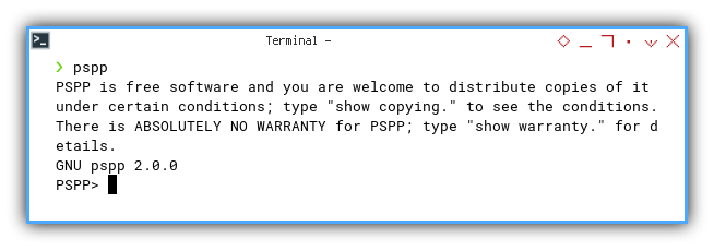
We need PSPPire to run the GUI (graphical user interface) Enter PSPPire for point-and-click joy. All the features of PSPP dressed up in windows and buttons.

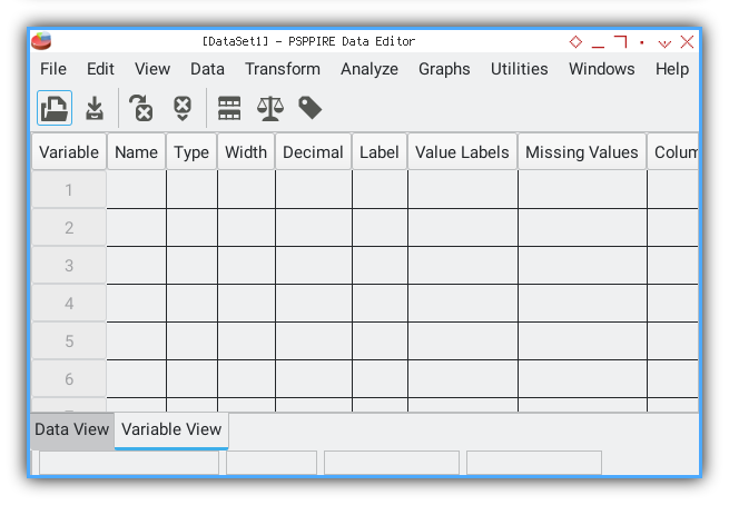
A GUI reduces the learning curve. We spend fewer brain cycles on syntax and more on interpreting p-values.

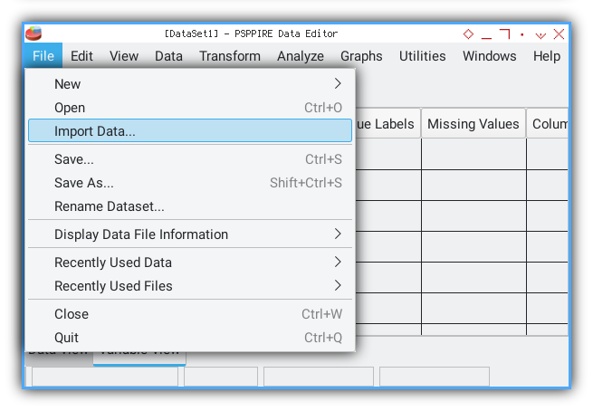
2: Import Data

Let’s bring in our trusty CSV of (x, y) pairs. We use the Import Data menu and follow PSPPire’s prompts. For example this CSV file

x, y
0, 5
1, 12
2, 25
3, 44
4, 69
5, 100
6, 137
7, 180
8, 229
9, 284
10, 345
11, 412
12, 485

File → Import Data → CSV

We point PSPPire at 50-samples.csv.

We need to follow required procedure, such as selecting rows.

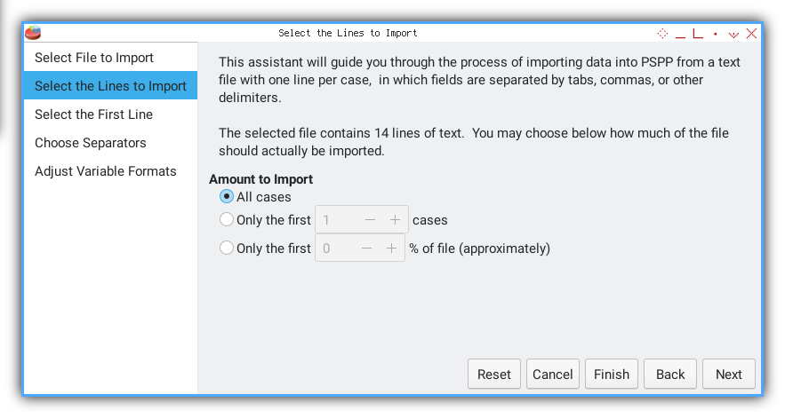
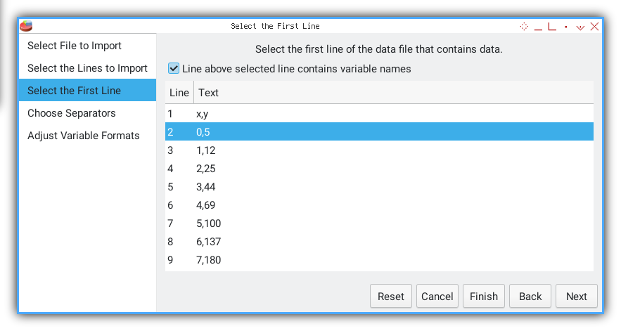
Select Data Start

We skip the header row and pick line 2 as first case.

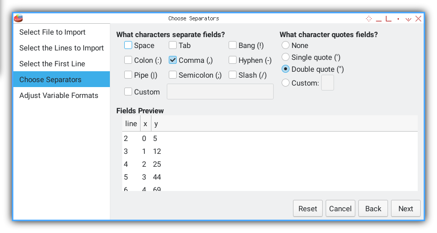
Choose Delimiter

Separator.

A comma tells PSPPire where one number ends and the next begins.

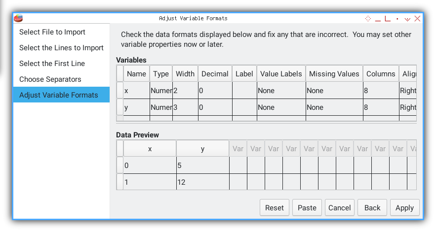
Define Variables

Variable format.

We assign x F2.0 and y F3.0 formats, enough precision for point plots.

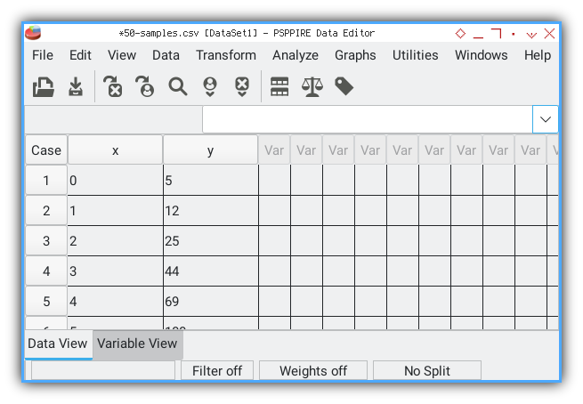
Data View

Once complete, the Data View shows our numbers in a grid.

PSPPire also spits out the equivalent PSPP command syntax in the Output Viewer:

GET DATA
  /TYPE=TXT
  /FILE="/home/epsi/50-samples.csv"
  /ARRANGEMENT=DELIMITED
  /DELCASE=LINE
  /FIRSTCASE=2
  /DELIMITERS=","
  /VARIABLES=
    x F2.0
    y F3.0.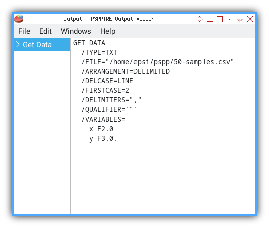

The output above is the command line.

Having the generated command gives us reproducibility, and a behind-the-scenes peek at PSPP’s underbelly. If we ever need to automate or script a batch of files, we already have the template.

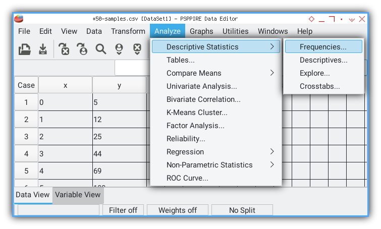
3: Frequency Analysis

With our data safely in PSPPire, we can summon a full suite of descriptive statistics in just a few clicks. Now you can do analysis easily.

Running Frequencies

Analysis → Frequencies

We select variables x and y to analyze, using analysis menu.

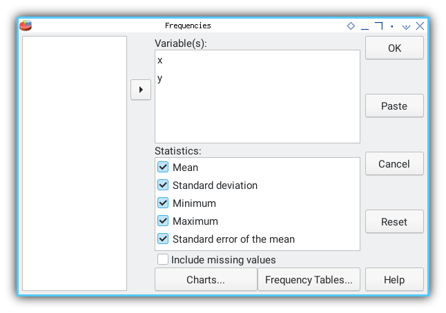
Dialog Settings

We check options for tables and all statistics. Then click OK.

Output Viewer

In an instant PSPPire serves up our results in the Output Viewer.

Behind the Scenes: PSPP Syntax

PSPPire graciously shows us the equivalent command syntax, so we know exactly what happened under the hood:

FREQUENCIES
	/VARIABLES= x y
	/FORMAT=AVALUE TABLE
	/STATISTICS=ALL.

Seeing the command ensures our analysis is reproducible. We can save or tweak it later for batch processing, no mystery clicks required.

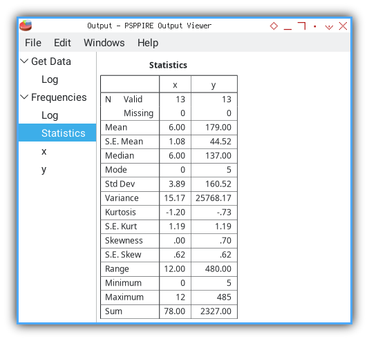
The Table of Truth

PSPPire lays out all the key properties we calculated earlier. Here’s a condensed view:

        Statistics
╭─────────┬─────┬────────╮
│         │  x  │    y   │
├─────────┼─────┼────────┤
│N Valid  │   13│      13│
│  Missing│    0│       0│
├─────────┼─────┼────────┤
│Mean     │ 6.00│  179.00│
├─────────┼─────┼────────┤
│S.E. Mean│ 1.08│   44.52│
├─────────┼─────┼────────┤
│Median   │ 6.00│  137.00│
├─────────┼─────┼────────┤
│Mode     │    0│       5│
├─────────┼─────┼────────┤
│Std Dev  │ 3.89│  160.52│
├─────────┼─────┼────────┤
│Variance │15.17│25768.17│
├─────────┼─────┼────────┤
│Kurtosis │-1.20│    -.73│
├─────────┼─────┼────────┤
│S.E. Kurt│ 1.19│    1.19│
├─────────┼─────┼────────┤
│Skewness │  .00│     .70│
├─────────┼─────┼────────┤
│S.E. Skew│  .62│     .62│
├─────────┼─────┼────────┤
│Range    │12.00│  480.00│
├─────────┼─────┼────────┤
│Minimum  │    0│       5│
├─────────┼─────┼────────┤
│Maximum  │   12│     485│
├─────────┼─────┼────────┤
│Sum      │78.00│ 2327.00│
╰─────────┴─────┴────────╯

In one neat table we confirm sample size, missing data, central tendency dispersion shape and range. It’s our statistical Swiss army knife.

Verify Excel

Cross-Tool Verification

You may compare the result, with our previous calculation with Excel.

Our built-in formulas produced identical means medians variances and so on.

Verify Python

Cross-Tool Verification

You may compare the result, with our previous calculation with Python.

Our numpy scipy script echoed the same results:

x (max, min, range) = (   0.00,   12.00,   12.00 )
y (max, min, range) = (   5.00,  485.00,  480.00 )

x median       =      6.00
y median       =    137.00
x mode         =      0.00
y mode         =      5.00

x kurtosis     =     -1.20
y kurtosis     =     -0.73
x skewness     =      0.00
y skewness     =      0.70

x SE kurtosis  =      1.19
y SE kurtosis  =      1.19
x SE skewness  =      0.62
y SE skewness  =      0.62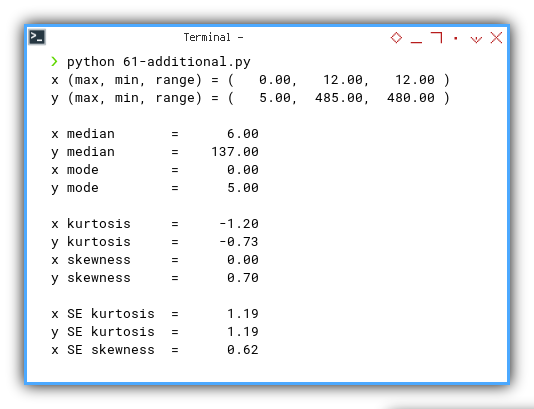

When three independent tools agree we can trust our numbers. Discrepancies would signal a bug or a typo.

4: Linear Regression Analysis

We can harness PSPPire to run a full linear regression in a few clicks. Let us see how our GUI stacks up against spreadsheets and scripts.

Running the Regression

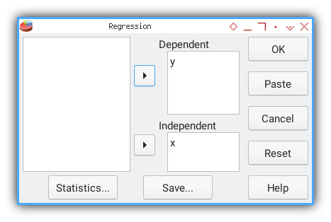
Analysis → Regression → Linear

Again, fill the necessary dialog. We assign x as predictor and y as dependent. Then click OK.

Output Viewer

PSPPire serves up tables for model summary, ANOVA, and coefficients. No calculator required.

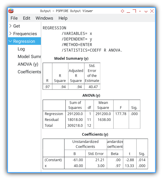
A built-in regression procedure frees us from manual formula work, and ensures consistency with standard statistical methods.

PSPP Command Syntax

PSPPire logs the equivalent command so we can script this later:

REGRESSION
	/VARIABLES= x
	/DEPENDENT= y
	/METHOD=ENTER
	/STATISTICS=COEFF R ANOVA.

Seeing the command offers reproducibility. We can batch process multiple datasets by tweaking one script.

Model Summary

PSPPire’s Model Summary matches our earlier calculations, for R, R², adjusted R², and standard error of estimate:

                     Model Summary (y)
╭───┬────────┬─────────────────┬──────────────────────────╮
│ R │R Square│Adjusted R Square│Std. Error of the Estimate│
├───┼────────┼─────────────────┼──────────────────────────┤
│.97│     .94│              .94│                     40.47│
╰───┴────────┴─────────────────┴──────────────────────────╯

This table tells us how well x explains y. An R² of 0.94 means 94% of variance in y is captured by our linear model.

ANOVA Table

Next PSPPire gives us ANOVA details: sums of squares, degrees of freedom, mean squares, F statistic, and significance:

                       ANOVA (y)
╭──────────┬──────────────┬──┬───────────┬──────┬────╮
│          │Sum of Squares│df│Mean Square│   F  │Sig.│
├──────────┼──────────────┼──┼───────────┼──────┼────┤
│Regression│      291200.0│ 1│   291200.0│177.78│.000│
│Residual  │      18018.00│11│    1638.00│      │    │
│Total     │      309218.0│12│           │      │    │
╰──────────┴──────────────┴──┴───────────┴──────┴────╯

The huge F value and p-value < 0.001 confirm that, our regression model is statistically significant.

Coefficients

Finally we see the unstandardized and standardized coefficients, their standard errors, t-values, and significance:

                               Coefficients (y)
╭──────────┬────────────────────────────┬─────────────────────────┬─────┬────╮
│          │ Unstandardized Coefficients│Standardized Coefficients│     │    │
│          ├────────────┬───────────────┼─────────────────────────┤     │    │
│          │      B     │   Std. Error  │           Beta          │  t  │Sig.│
├──────────┼────────────┼───────────────┼─────────────────────────┼─────┼────┤
│(Constant)│      -61.00│          21.21│                      .00│-2.88│.014│
│x         │       40.00│           3.00│                      .97│13.33│.000│
╰──────────┴────────────┴───────────────┴─────────────────────────┴─────┴────╯

Coefficient B = 40 tells us that, for each one-unit increase in x, y, increases by 40 on average.

The intercept −61 and its p-value let us judge, whether the line truly crosses zero meaningfully.

Verify Excel

Cross-Tool Verification

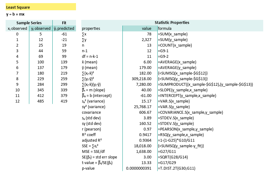
You may compare the result, with our previous calculation with excel and python. Our tabular worksheet yielded identical slope, intercept, t-value, and standard errors.

And also the right part of the worksheet.

Verify Python

Cross-Tool Verification

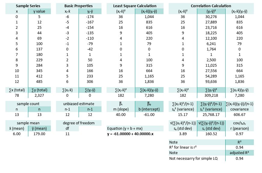
You may compare the result, with our previous calculation with Python. Our numpy/scipy calculations match PSPPire’s output:

n          =   13
∑x (total) =   78.00
∑y (total) = 2327.00
x̄ (mean)   =    6.00
ȳ (mean)   =  179.00

∑(xᵢ-x̄)    =      0.00
∑(yᵢ-ȳ)    =      0.00
∑(xᵢ-x̄)²   =    182.00
∑(yᵢ-ȳ)²   = 309218.00
∑(xᵢ-x̄)(yᵢ-ȳ)  =   7280.00
m (slope)      =     40.00
b (intercept)  =    -61.00

Equation     y = -61.00 + 40.00.x

sₓ² (variance) =     14.00
sy² (variance) =  23786.00
covariance     =    560.00
sₓ (std dev)   =      3.74
sy (std dev)   =    154.23
r (pearson)    =      0.97
R²             =      0.94

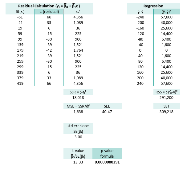
SSR = ∑ϵ²           =  18018.00
MSE = ∑ϵ²/(n-2)     =   1638.00
SE(β₁)  = √(MSE/sₓ) =      3.00
t-value = β̅₁/SE(β₁) =     13.33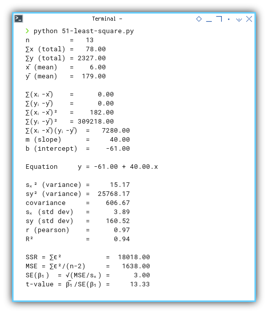

Agreement across Excel, Python, and PSPPire confirms, that no computations are off. We can trust these regression estimates.

5: Polynomial Regression Analysis

Using Shell

After getting comfortable with PSPPire, let’s go full command line, trade the GUI for a keyboard only experience. The PSPP terminal gives us more flexibility, than the point-and-click world. And yes, we can run polynomial regression right here in the shell.

Data Source

Let’s try a new dataset.

xs, ys1, ys2, ys3
0,  5,   5,   5
1,  9,   12,  14
2,  13,  25,  41
3,  17,  44,  98
4,  21,  69,  197
5,  25,  100, 350
6,  29,  137, 569
7,  33,  180, 866
8,  37,  229, 1253
9,  41,  284, 1742
10, 45,  345, 2345
11, 49,  412, 3074
12, 53,  485, 3941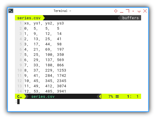

We’ll focus on xs and ys3, but feel free to explore the other columns too. They’re not just filler, they’re backup dancers.

Import Data

Here’s how we get our data into PSPP shell. The command is simple, nothing fancy. This time we have four columns.

GET DATA
  /TYPE=TXT
  /FILE="/home/epsi/series.csv"
  /ARRANGEMENT=DELIMITED
  /DELCASE=LINE
  /FIRSTCASE=2
  /DELIMITERS=","
  /VARIABLES=
    xs F2.0
    ys1 F2.0
    ys2 F3.0
    ys3 F4.0.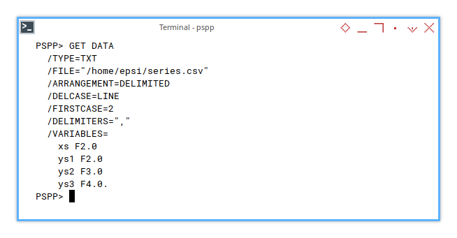

Statistic Properties

Check the Metrics

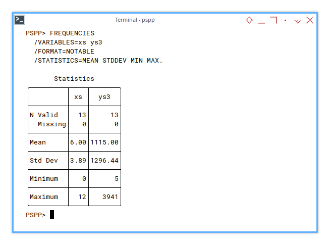
Before we dive into curves, let’s get a sense of scale. This time only what we need.: Mean, standard deviation, min, max.

FREQUENCIES
  /VARIABLES=xs ys3
  /FORMAT=NOTABLE
  /STATISTICS=MEAN STDDEV MIN MAX.

With the result as below:

       Statistics
╭─────────┬────┬───────╮
│         │ xs │  ys3  │
├─────────┼────┼───────┤
│N Valid  │  13│     13│
│  Missing│   0│      0│
├─────────┼────┼───────┤
│Mean     │6.00│1115.00│
├─────────┼────┼───────┤
│Std Dev  │3.89│1296.44│
├─────────┼────┼───────┤
│Minimum  │   0│      5│
├─────────┼────┼───────┤
│Maximum  │  12│   3941│
╰─────────┴────┴───────╯

Polynomial Regression Coefficient

Quadratic

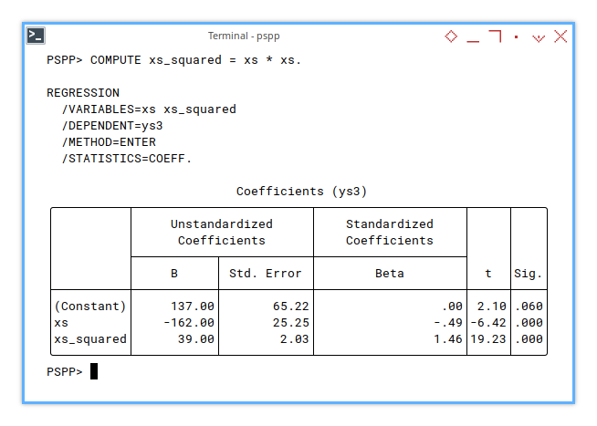
To compute polynomial regression, we need to define xs² helper variable first. This turns our linear regression into something a bit curvier.

COMPUTE xs_squared = xs * xs.

REGRESSION
  /VARIABLES=xs xs_squared
  /DEPENDENT=ys3
  /METHOD=ENTER
  /STATISTICS=COEFF.

And we get:

                              Coefficients (ys3)
╭──────────┬────────────────────────────┬─────────────────────────┬─────┬────╮
│          │ Unstandardized Coefficients│Standardized Coefficients│     │    │
│          ├────────────┬───────────────┼─────────────────────────┤     │    │
│          │      B     │   Std. Error  │           Beta          │  t  │Sig.│
├──────────┼────────────┼───────────────┼─────────────────────────┼─────┼────┤
│(Constant)│      137.00│          65.22│                      .00│ 2.10│.060│
│xs        │     -162.00│          25.25│                     -.49│-6.42│.000│
│xs_squared│       39.00│           2.03│                     1.46│19.23│.000│
╰──────────┴────────────┴───────────────┴─────────────────────────┴─────┴────╯

It matches our results in Excel/Calc and Python. Harmony across platforms, every data analyst’s dream.

Cubic

Let’s go one degree hotter, cubic regression with xs² and xs³. Add a third power term and suddenly we’re modeling rollercoasters.

COMPUTE xs_squared = xs * xs.
COMPUTE xs_cubed = xs * xs * xs.

REGRESSION
  /VARIABLES=xs xs_squared xs_cubed
  /DEPENDENT=ys3
  /METHOD=ENTER
  /STATISTICS=COEFF.

And here’s the result:

                                Coefficients (ys3)
╭──────────┬────────────────────────────┬─────────────────────────┬────────┬────╮
│          │ Unstandardized Coefficients│Standardized Coefficients│        │    │
│          ├───────────┬────────────────┼─────────────────────────┤        │    │
│          │     B     │   Std. Error   │           Beta          │    t   │Sig.│
├──────────┼───────────┼────────────────┼─────────────────────────┼────────┼────┤
│(Constant)│       5.00│             .00│                      .00│+Infinit│.000│
│xs        │       4.00│             .00│                      .01│+Infinit│.000│
│xs_squared│       3.00│             .00│                      .11│+Infinit│.000│
│xs_cubed  │       2.00│             .00│                      .88│+Infinit│.000│
╰──────────┴───────────┴────────────────┴─────────────────────────┴────────┴────╯

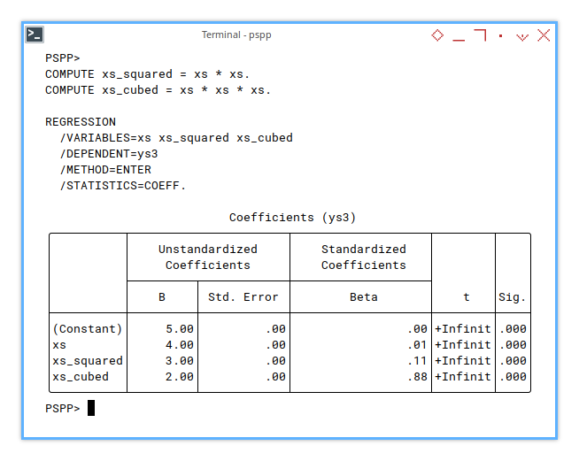
Still consistent with our Excel/Calc and Python results.

Do you think that the variable format is very similar to LINEST formula?
Do you think that this similarity has to do with design matrix?

That’s the power of methodical math. We can call this replication, but it feels more like statistical déjà vu.

Beyond Regression

Easy peasy? Don’t be so sure.

If all we needed were the coefficients, we could stop here and call it a day. But PSPP (and its big sibling SPSS) are statistical beasts, with much more beneath the surface. We’ve only tiptoed into the shallow end.

There’s a world of diagnostics, assumptions, plots, and tests ahead. Think of this as checking your tire pressure before a race. Important, but far from the whole event.

Now that we’ve done our part:

exit.

Stay humble, statisticians.

• The more we explore, the clearer it becomes, we’ve only just touched the surface.

• In the sea of statistics, every method we master reveals deeper waters ahead.

• Moving from spreadsheets to statistical tools, we realize how vast the field truly is.

• No matter how far we’ve come, there’s always more to learn.

Stay humble!

What’s Next for Our Curious Clipboard? 📋

We’ve poked around PSPPire, ran some regressions, and even peeked under the hood at those ANOVA pistons firing. But where do we steer our statistical engine next? Let’s break it down—three lanes ahead.

Further Analysis

PSPPire Knows More Than It Shows

If we regularly wrestle with data, PSPP is not just a friend. It’s the nerdy lab partner who finishes our sentences with a p-value. PSPPire offers way more than we’ve explored here, from nonparametric tests to factor analysis, but diving into every nook would require another trilogy.

Let’s be honest. This article was never meant to be a full tour of PSPPire. Think of it as a strong cup of coffee, and a friendly push into the statistics playground. The rest? Explore when the data screams louder, or when our spreadsheet starts judging us.

Mastering the basics lets us decide, when to trust software and when to double-check. Knowing the tools means we’re never stuck, staring at an error bar like it’s an existential crisis.

The Curiosities We Skipped (But Might Revisit)

What’s left behind 🤔?

Yes, we did regression. We danced with the line of best fit. We even toyed with quadratic and cubic forms, like high schoolers rewriting song lyrics into parabolas.

But we skipped a few gems:

• What if we measured correlation, between two datasets on the same x-axis?

• Or looked at how the fluctuation of one variable, predicts the fluctuation of another? Think of it as emotional intelligence for spreadsheets.

And we haven’t touched splines. Because honestly, splines are the deep-fried snacks of stats. Delicious but hard to digest without proper guidance.

Regression is just the beginning. Real-world data is rarely linear and never polite. These advanced approaches let us understand, when data moves together, when it rebels, and when it just wants to be left alone.

Other Languages, Same Obsession

Sure, we’ve dabbled in Python. But the statistical family dinner is much bigger:

• R: The grandmaster of stats. It comes with more packages than a post office in December.

• Julia: Lightning-fast and math-savvy. For those who want to feel both trendy and efficient.

• Go: For when we need stats to run inside a production-grade backend, and still sleep well at night.

Choosing a language is like picking a wrench. The goal isn’t to be fancy. It’s to make the data talk, and sometimes scream.

Feeling adventurous? Join us in the next article: 👉 [ Trend - Language - R - Part One ]