Preface
Goal: Pretty statistics visualization with Seaborn, equipped with example script for each plots.
Let’s face it: plotting raw numbers in matplotlib is,
like eating plain oatmeal. Nutritious but a little… bland.
Enter Seaborn, the library that dresses our data in a tuxedo,
adds a spotlight, and whispers the punchline for you.
In this article, we will find ready-to-run example scripts for each plot. No tedious step-by-step handholding (the internet’s already brimming with tutorials). Our mission is to showcase what Seaborn can do for our statistical properties, so we can spend less time wrestling with code, and more time interpreting elegant visuals.
Remember: real-world data rarely stays neat and tidy. These are simple demos, consider them our rehearsal dinner before the big data wedding. Now, grab our favorite beverage and let’s our Seaborn’s stat-smarts in action.
Visualizing Linear Regression
Yes, we are still talking about trend, now with Seaborn.
Data Series
Instead of just one series,
we’ll play with these three: ys₁, ys₂, or ys₃.
That way we can compare how different curves behave side by side.
xs, ys1, ys2, ys3
0,  5,   5,   5
1,  9,   12,  14
2,  13,  25,  41
3,  17,  44,  98
4,  21,  69,  197
5,  25,  100, 350
6,  29,  137, 569
7,  33,  180, 866
8,  37,  229, 1253
9,  41,  284, 1742
10, 45,  345, 2345
11, 49,  412, 3074
12, 53,  485, 3941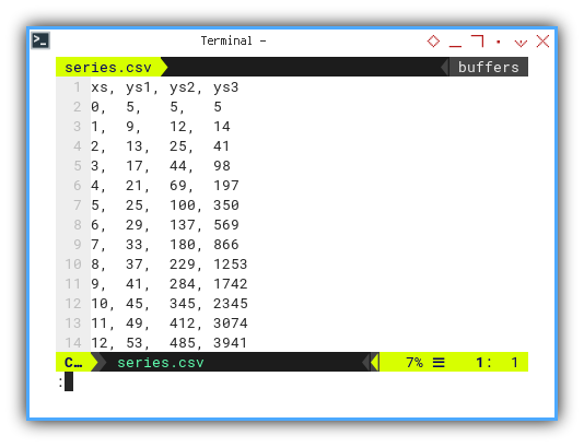
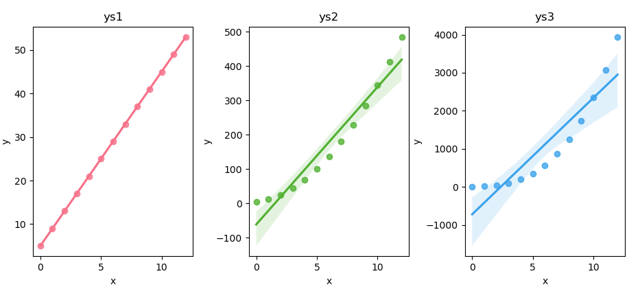
Comparing multiple series in one plot helps us, see at a glance which trendlines are stubbornly linear, and which ones go off to dramatic nonlinear land.
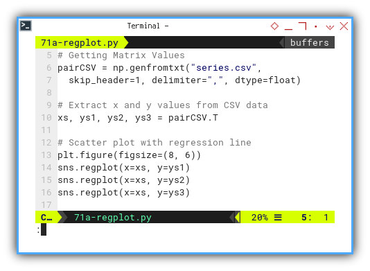
Regression Plot
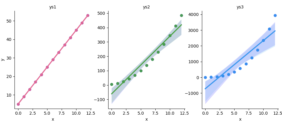
A simple way to overlay regression lines, on scatter points for each series. Plotting linear regression plot is straightforward. We can plot all these three series at once in one plot figure.
# Getting Matrix Values
pairCSV = np.genfromtxt("series.csv",
  skip_header=1, delimiter=",", dtype=float)

# Extract x and y values from CSV data
xs, ys1, ys2, ys3 = pairCSV.T

# Scatter plot with regression line
plt.figure(figsize=(8, 6))
sns.regplot(x=xs, y=ys1)
sns.regplot(x=xs, y=ys2)
sns.regplot(x=xs, y=ys3)
With one command per series we get data points, regression line, and confidence band. It’s like magic, but with math under the hood.
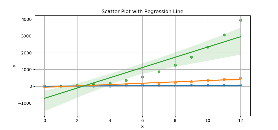
The result of the plot can be visualized as below:
You can obtain the interactive JupyterLab in this following link:
Or if you wish you can have three subplots in one figure with the help of tight layout,
Three-in-One Subplots
When overlaying clutters the view, we can split into three panels, all neatly aligned.
Prepare our data first. Getting Matrix Values, and extract x and y values from CSV data.
pairCSV = np.genfromtxt("series.csv",
  skip_header=1, delimiter=",", dtype=float)

xs, ys1, ys2, ys3 = pairCSV.T
Create the subplots. And also defining seaborn color palette. You can specify the number of colors here.
# Creating subplots
fig, axs = plt.subplots(1, 3, figsize=(12, 4))

palette = sns.color_palette("husl", 3)
Then plotting each scatter plot with regression line.
pairs = zip([ys1, ys2, ys3], ['ys1', 'ys2', 'ys3'])

for i, (ys, title) in enumerate(pairs):
  sns.regplot(x=xs, y=ys,
    ax=axs[i], color=palette[i])

  axs[i].set_title(title)
  axs[i].set_xlabel('x')
  axs[i].set_ylabel('y')

plt.tight_layout()
plt.show()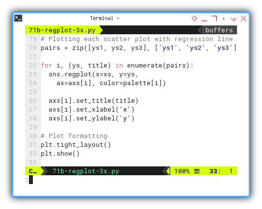
The result of the plot can be visualized as follows. All with pretty color. You can see the color is better than matplotlib.
You can obtain the interactive JupyterLab in this following link:
Side-by-side panels make it easy,
to compare slopes and scatter spread across series.
Plus the colors from husl give our eyes a treat.
Linear Model Plot
LM: Linear Model
Leverage lmplot for a concise call,
that handles DataFrame melting and faceting under the hood.
We can make the code above simpler with lmplot.
With panda dataframe, we can read data from CSV directly. But beware of the strip leading spaces from column names.
Before using the dataframe,
we need to transform the DataFrame to long format for linear model plot.
We can do this using melt method from panda.
df = pd.read_csv("series.csv") \
  .rename(columns=lambda x: x.strip())

df_melted = pd.melt(df,
  id_vars='xs', var_name='y', value_name='value')
Then we can draw scatter plot with regression line. For convenience, I adjust the title position a bit, so the title fit in small sized figure.
plt.figure(figsize=(8, 6))
sns.lmplot(x='xs', y='value',
  data=df_melted, hue='y')

plt.subplots_adjust(top=0.9)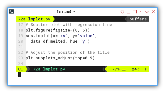
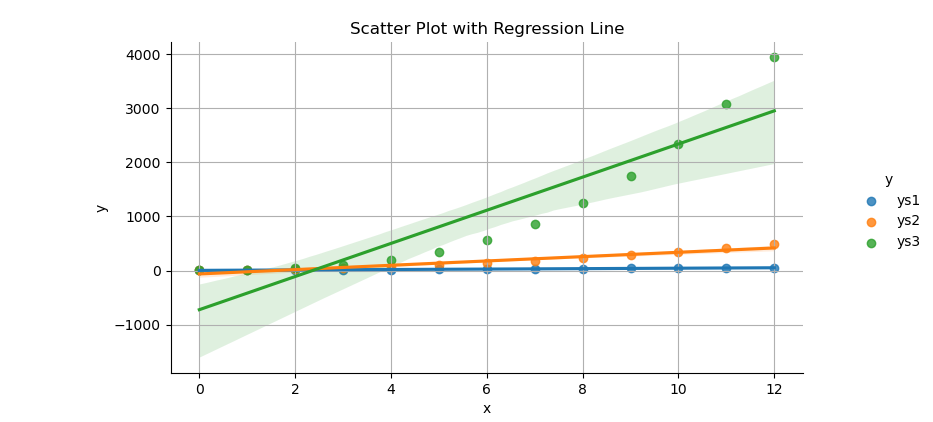
The result of the plot can be visualized as below:
You can obtain the interactive JupyterLab in this following link:
lmplot combines regression, hue-based grouping,
and faceting in one shot.
It’s the Swiss Army knife of trend visualization.
Facet Grid
Grid of Plot
For ultimate control we can use FacetGrid,
for multiple subplots sharing axes or not.
Instead of using subplots,
we can arrange our plot in a grid.
I give you two different examples.
One with shared y-axis,
and the other having different y-axis for each.
First we need to get the matrix values.
Then convert the values to pandas dataframe.
For use with this facetgrid,
we need to melt the dataframe to long format.
pairCSV = np.genfromtxt("series.csv",
  skip_header=1, delimiter=",", dtype=float)

cols_all = ['xs', 'ys1', 'ys2', 'ys3']
cols_sel = ['ys1', 'ys2', 'ys3']

df = pd.DataFrame(pairCSV, columns=cols_all)

df_melted = pd.melt(df,
  id_vars='xs', var_name='y', value_name='value')
Or share the y-axis and vary x-axis limits.
We need to create a facetgrid with one row and three columns,
with different y-axis for each.
Then we can map regplot to each facet.
g = sns.FacetGrid(df_melted,
  col='y', col_wrap=3, height=4, sharey=False)

g.map_dataframe(sns.regplot,
  x='xs', y='value', color='b')
We can iterate over selected columns and
map regplot to each column in the facetgrid.
In the iteration,
we should filter dataframe subset for each ys category.
Also for each ys category we can use different color,
based on sns.color_palette.
for ax, ys_name in zip(g.axes.flat, cols_sel):
  df_subset = df_melted[
    df_melted['y'] == ys_name]

  color = sns.color_palette("husl", 3)[
    cols_sel.index(ys_name)]

  sns.regplot(x='xs', y='value',
    data=df_subset, ax=ax,
    color=color)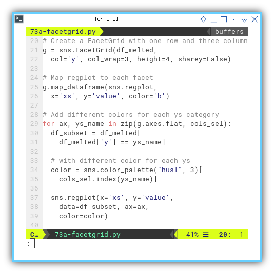
The result of the plot can be visualized as below. They all shared the same y-axis.
You can obtain the interactive JupyterLab in this following link:
If you want you can have different y-axis for each grid.
With panda dataframe,
we can read data from CSV directly.
Do not firget to strip leading spaces from column names.
Now we define selected columns for ys series.
df = pd.read_csv("series.csv") \
  .rename(columns=lambda x: x.strip())

cols_sel = ['ys1', 'ys2', 'ys3']
As usual we should melt the DataFrame to long format for facetgrid.
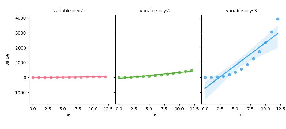
So we can create a facetgrid with seaborn
df_melted = df.melt(
  id_vars='xs', value_vars=cols_sel)

g = sns.FacetGrid(df_melted,
  col='variable', col_wrap=3,
  sharex=False, sharey=True)
Like previous example, we can iterate over selected columns and
map regplot to each column in the facetgrid.
for ax, col in zip(g.axes.flatten(), cols_sel):
  df_subset = df.melt(
    id_vars='xs', value_vars=col)

  color = sns.color_palette("husl", 3)[
    cols_sel.index(col)]

  sns.regplot(x='xs', y='value',
    data=df_subset, ax=ax, color=color)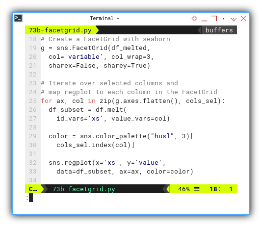
The result of the plot can be visualized as below:
You can obtain the interactive JupyterLab in this following link:
FacetGrid is our multi-paneled stage. We decide whether our subplots share scales or stand alone, giving us granular control over comparisons.
Visualizing Statistics Properties
We have four plots that share almost identical setup. Each one gives us a different lens on the same data Let’s prepare our data once and then explore:
- Boxplot
- Violinplot
- Swarmplot
- Striplot
Preparing Dataframe
These plot required the the same data preparation.
As usual, you might either read the dataframe from panda directly,
or using numpy’s np.genfromtxt.
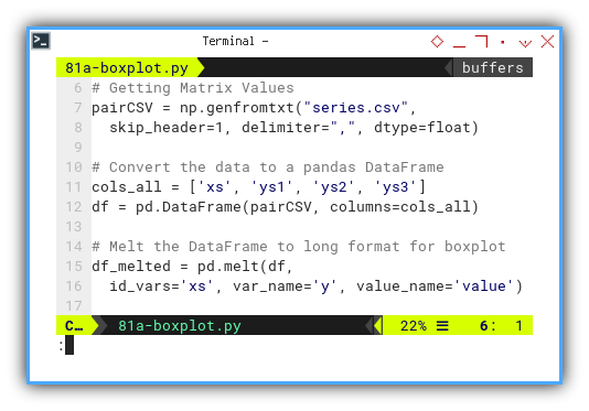
First we need to get the matrix values. Then convert the values to pandas dataframe. For use with this these four kinds of plot, we need to melt the dataframe to long format.
pairCSV = np.genfromtxt("series.csv",
  skip_header=1, delimiter=",", dtype=float)

cols_all = ['xs', 'ys1', 'ys2', 'ys3']
df = pd.DataFrame(pairCSV, columns=cols_all)

df_melted = pd.melt(df,
  id_vars='xs', var_name='y', value_name='value')
We load the CSV, convert to a DataFrame, and melt it into long form. This step powers every plot below.
One tidy DataFrame fuels many plots. We avoid copy paste and ensure consistency across visuals.
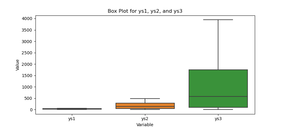
Box Plot
The box plot is the classic. It shows median quartiles and outliers at a glance.
Creating boxplot is as simple as below:
plt.figure(figsize=(8, 6))
sns.boxplot(x='y', y='value', data=df_melted)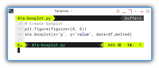
The result of the plot can be visualized as below:
You can obtain the interactive JupyterLab in this following link:
Box plots highlight center spread and extreme points. If a whisker goes rogue we notice immediately.
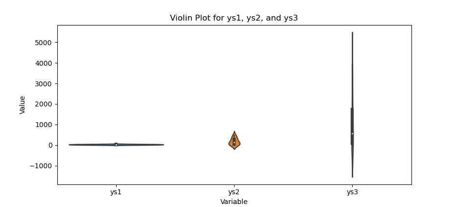
Violin Plot
Violin plots layer a kernel density estimate, around the box plot structure for extra flair. This is basically the sum of normal distribution.
Creating violinplot is also simple.
plt.figure(figsize=(8, 6))
sns.violinplot(x='y', y='value', data=df_melted)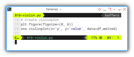
The result of the plot can be visualized as below:
You can obtain the interactive JupyterLab in this following link:
Violin plots reveal the full distribution shape. We see multimodal bumps or smooth bell curves at a glance.
Swarm Plot
Swarm plots show individual observations while avoiding overlap. It’s like inviting each data point to stand in its own space.
We can define colors for swarmplot,
by adjust the number of colors as needed,
so we can create swarmplot with different colors
colors = sns.color_palette("husl", 3)

plt.figure(figsize=(8, 6))
sns.swarmplot(x='y', y='value',
  hue='y', data=df_melted, palette=colors)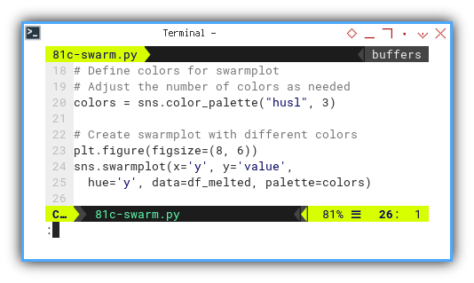
The result of the plot can be visualized as below:
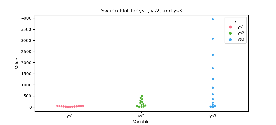
You can obtain the interactive JupyterLab in this following link:
Swarm plots let us see the actual data points. We spot clusters, gaps, and any singletons that box or violin plots might hide.
Strip Plot
Strip plots are like swarms but allow us, to dodge points side by side. They give a sense of overlap density.
Just like swarmplot,
We can define colors by adjust the number of colors as needed,
so we can create the striplot with different colors
colors = sns.color_palette("husl", 3)

plt.figure(figsize=(8, 6))
sns.stripplot(x='y', y='value', data=df_melted,
  hue='y', palette=colors, dodge=True)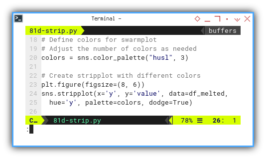
The result of the plot can be visualized as below:
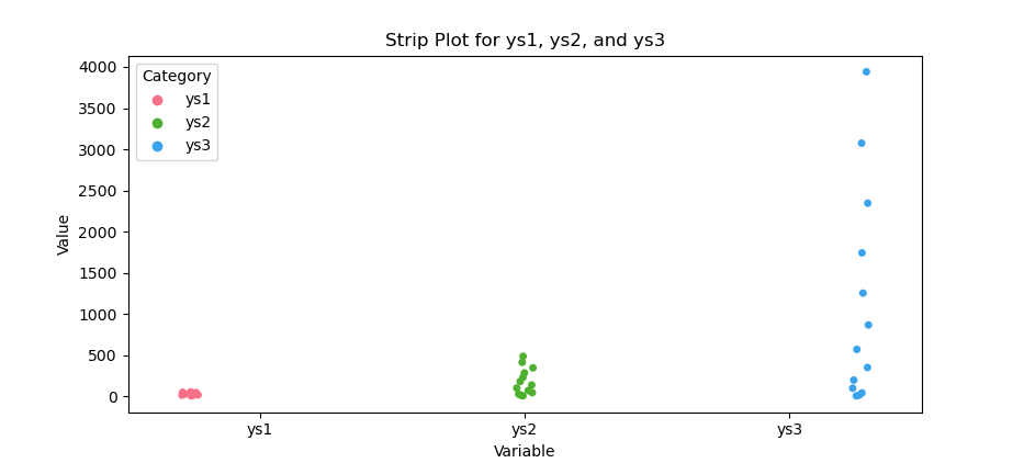
You can obtain the interactive JupyterLab in this following link:
Strip plots combine the clarity of swarm plots with grouping dodge. We see individual values and group separation at once.
Visualizing Distribution
When it comes to distribution plots, Seaborn makes our lives a breeze. We get beautiful charts with minimal code, and maximum statistical insight.
KDE Plot
Kernel Density Estimation
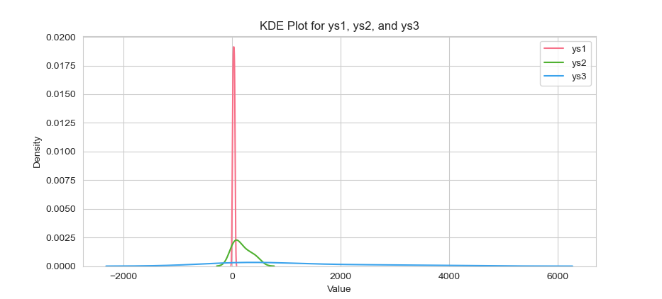
Kernel Density Estimation turns each data point, into a little bell curve and sums them all together. The result is a smooth silhouette of our data’s true shape.
This is the sum of normal distribution for each points for a data series.
As usual we can prepare the data. Then seaborn decoration such as the style. And also define a color palette for the KDE plot, with adjustable number of colors as you needed.
df = pd.read_csv("series.csv") \
  .rename(columns=lambda x: x.strip())

sns.set_style("whitegrid")
palette = sns.color_palette("husl", 3)

plt.figure(figsize=(8, 6))
And create a KDE plot for each ys category.
for i, col in enumerate(['ys1', 'ys2', 'ys3']):
  sns.kdeplot(data=df[col],
    color=palette[i], label=col)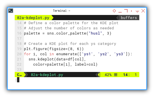
The result of the plot can be visualized as below:
You can obtain the interactive JupyterLab in this following link:
If you wish, you can customize the style, with other parameters.
df = pd.read_csv("series.csv")
df_melted = pd.melt(df, id_vars='xs',
  var_name='Category', value_name='Value')

sns.set_style("darkgrid")

plt.figure(figsize=(8, 6))
Then we can create KDE plot for all categories with oneliner settings.
sns.kdeplot(data=df_melted,
  x='Value', hue='Category', palette='deep',
  alpha=0.7, multiple='stack', linewidth=2)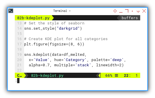
The result of the plot can be visualized as below:
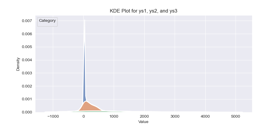
Customize further:
KDE plots reveal subtle bumps and tails that histograms can miss. They help us spot multimodal distributions or heavy tails in a flash.
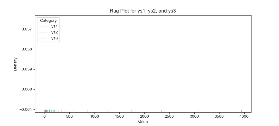
Rug Plot
Sometimes the simplest visualization is the most telling. A rug plot adds one tick for each observation. It’s like sprinkling sugar on a cake. Small but impactful.
As usual we need to melt the dataframe to long format for rugplot.
df = pd.read_csv("series.csv")

df_melted = pd.melt(df, id_vars='xs',
  var_name='Category', value_name='Value')
For decoration purpose we need to define a color palette for the rug plots. With using one less color for ‘xs’
palette = sns.color_palette(
  "husl", len(df.columns) - 1)

plt.figure(figsize=(8, 6))
Then we can create rug plot for each category, with ‘xs’ column excluded.
for i, col in enumerate(df.columns[1:]):
  df_subset = df_melted[df_melted['Category'] == col]
  sns.rugplot(data=df_subset, x='Value',
    color=palette[i], label=col, alpha=0.7)
The result of the plot can be visualized as below. This looks like an empty chart as first. But you can see the ticks at the below of the figure.
You can obtain the interactive JupyterLab in this following link:
Rug plots show raw data density without binning. They let us see exact observation locations and gaps in the data.
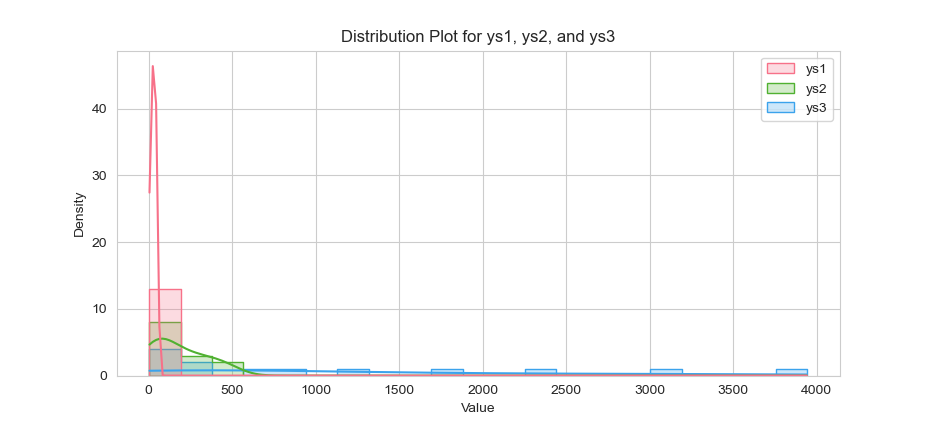
Histogram Plot
We all know histograms. So what is so special with this histogram? Seaborn’s histplot can add a KDE curve on top to combine the best of both worlds.
As usual we need to prepare data.
Then select columns such as ys₁, ys₂, and ys₃.
Then create a figure and axis objects.
df = pd.read_csv("series.csv") \
  .rename(columns=lambda x: x.strip())

cols_selected = ['ys1', 'ys2', 'ys3']

plt.figure(figsize=(8, 6))
This way we can plot displot for selected columns.
sns.histplot(data=df[cols_selected],
  kde=True, element='step',
  multiple='layer', palette='husl')
The result of the plot can be visualized as below:
Explore more:
Layering KDE on a histogram helps us, see both individual bin counts and the underlying density estimate. It’s clarity and style rolled into one.
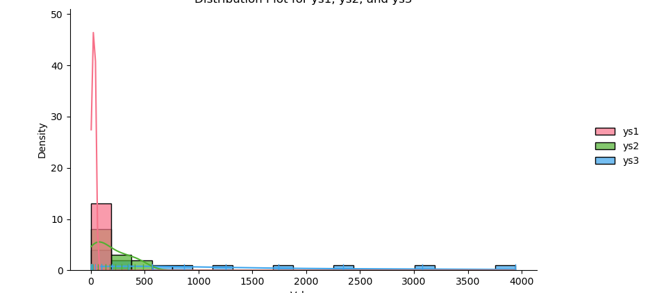
Distribution Plot
Seaborn’s displot ties it all together: histogram, KDE, and rug, into a single convenient function.
As above, we need to select columns,
such as ys₁, ys₂, and ys₃.
df = pd.read_csv("series.csv") \
  .rename(columns=lambda x: x.strip())

cols_selected = ['ys1', 'ys2', 'ys3']
df_selected = df[cols_selected]
Let’s decorate the figure as usual.
Defining a color palette for the displot.
palette = sns.color_palette(
  "husl", len(cols_selected))

plt.figure(figsize=(8, 6))
Now we can create displot for selected columns.
sns.displot(data=df_selected,
  kind='hist', rug=True, kde=True,
  palette=palette, alpha=0.7, multiple='layer')
The result of the plot can be visualized as below:
You can obtain the interactive JupyterLab in this following link:
displot is our all-in-one distribution toolkit.
It saves us boilerplate code and gives a comprehensive view of:
frequency, density, and individual data points.
Further Visualization
We can combine multiple layers of information into a single figure. For example these two plots add marginal distributions on the top and right sides, giving us both joint and individual views in one glance.
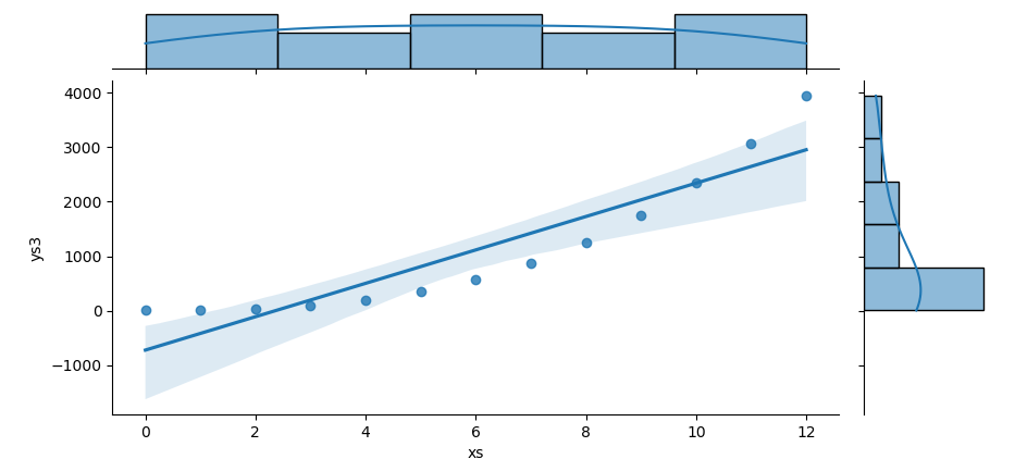
Joint Plot
Seaborn’s jointplot makes it trivial to pair a scatterplot with marginal density or histogram plots. Here we’ll illustrate a regression between xs and ys₃ with KDE filling on the margins.
For eaxmple, we can use seaborn’s jointplot
to create a scatter plot,
with KDE at the marginal.
df = pd.read_csv("series.csv") \
  .rename(columns=lambda x: x.strip())

sns.jointplot(data=df, x='xs', y='ys3',
  kind='reg', marginal_kws={'fill': True})
The result of the plot can be visualized as below:
You can obtain the interactive JupyterLab in this following link:
This plot shows both the relationship, between two variables and their individual distributions. We get regression insight and marginal shape in one compact view.
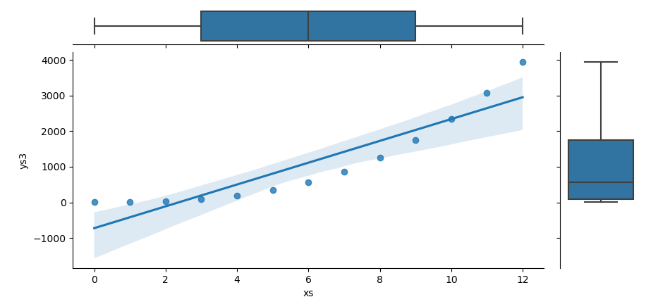
Joint Grid
For full customization we can build the same view by hand using JointGrid. This lets us choose any plot type for the center and the margins.
First we need to create a JointGrid object. Then plot the scatter plot in the center, and also set the histograms plot on the marginal axes.
df = pd.read_csv("series.csv") \
  .rename(columns=lambda x: x.strip())

g = sns.JointGrid(data=df, x='xs', y='ys3')
g.plot_joint(sns.regplot)
g.plot_marginals(sns.boxplot)
The result of the plot can be visualized as below:
You can obtain the interactive JupyterLab in this following link:
With JointGrid we control every layer. We can swap in histograms, violinplots, or any custom chart on the margins to suit our analysis needs.
What Comes Next 🤔?
We have dazzled our plots and explored distributions in all their glory. Now it is time to broaden our toolkit beyond Python and Seaborn.
I am eager to dive into PSPPire, the open source cousin of SPSS. It lets us run familiar statistical tests in a free, community-driven environment. Think of it as a statistical theme park, where all the rides are free and the cotton candy never runs out.
Learning PSPPire gives us another arrow in our quiver. When we need quick hypothesis tests or standardized reporting, PSPPire can deliver without licensing headaches.
Let us continue our adventure here: 🔗 [ Trend - Properties - PSPPire ].