Preface
Goal: Goes further from linear regression to polynomial regression. The practical implementation, shows how to execute the theory with spreadsheet.
Now that we’ve survived the theoretical terrain of polynomial regression (and our coffee mugs are still half full), it’s time to put numbers into cells and formulas into action.
Theory is where we understand, why fitting a 3rd-degree curve doesn’t mean we’re overfitting, necessarily. But practice is where we catch that overfit before it eats our model alive.
We’re going to:
-
Use both the
LINESTfunction and manual calculations. -
Start with raw cell references, to show what’s going on under the hood.
-
Later, evolve to named ranges, because
{=MMULT(E48:G50,E54:E56)}isn’t exactly readable poetry.
We want clarity, precision, and just a little flair. Think of it as data fashion: we’re not just dressing up the numbers. We’re making them walk the runway.
From theoretical foundations we are going shift to practical implementation in daily basis, using spreadsheet formula, python tools, and visualizations.
While the theory explains why the math works, the practice shows how to execute it with real tools. With the flow, from theory to tabular spreadsheets, then from we are going to build visualization using python.
We are going to use both linest formula and manual calculation.
We are going to start with simple cell address in formula,
avoiding complex spreadsheet feature.
Then we are going to continue by using named range,
simplifying the formula understanding,
by using name instead of plain cell address.
1: What the Sheet Does
And Why It Matters
The simplest way to get standard error from a polynomial regression in Excel?
Just summon the mighty =LINEST(y-range, x-range^{1,2,...,n}, TRUE, TRUE) formula.
Boom. Coefficients. Stats. Done.
But if you are the sort who reads footnotes and double-checks calculators, you might want to peek behind the curtain and replicate it manually.
Here’s the catch: unlike linear regression, Excel doesn’t hand you variance, covariance, and residuals on a silver platter for higher-order polynomials. We’re on our own.
Fear not! We’re already armed. The previous articles gave us the mathematical gear, we just need to wield it.
Worksheet Source
The Artefact of Polynomial Power
You can download and dissect the Excel file used in this article. It’s ready for experimentation, and yes, feel free to break it. That’s how breakthroughs happen.
Basic Stuff
Nomore spoon-feeding.
If you’ve followed along this far, chances are your spreadsheet reflexes are already warmed up.
This sheet builds directly on the formulas introduced in:
So no hand-holding here. Instead of step-by-step spoon-feeding, we’ll do brief overviews for each section, like a cooking show for regression.
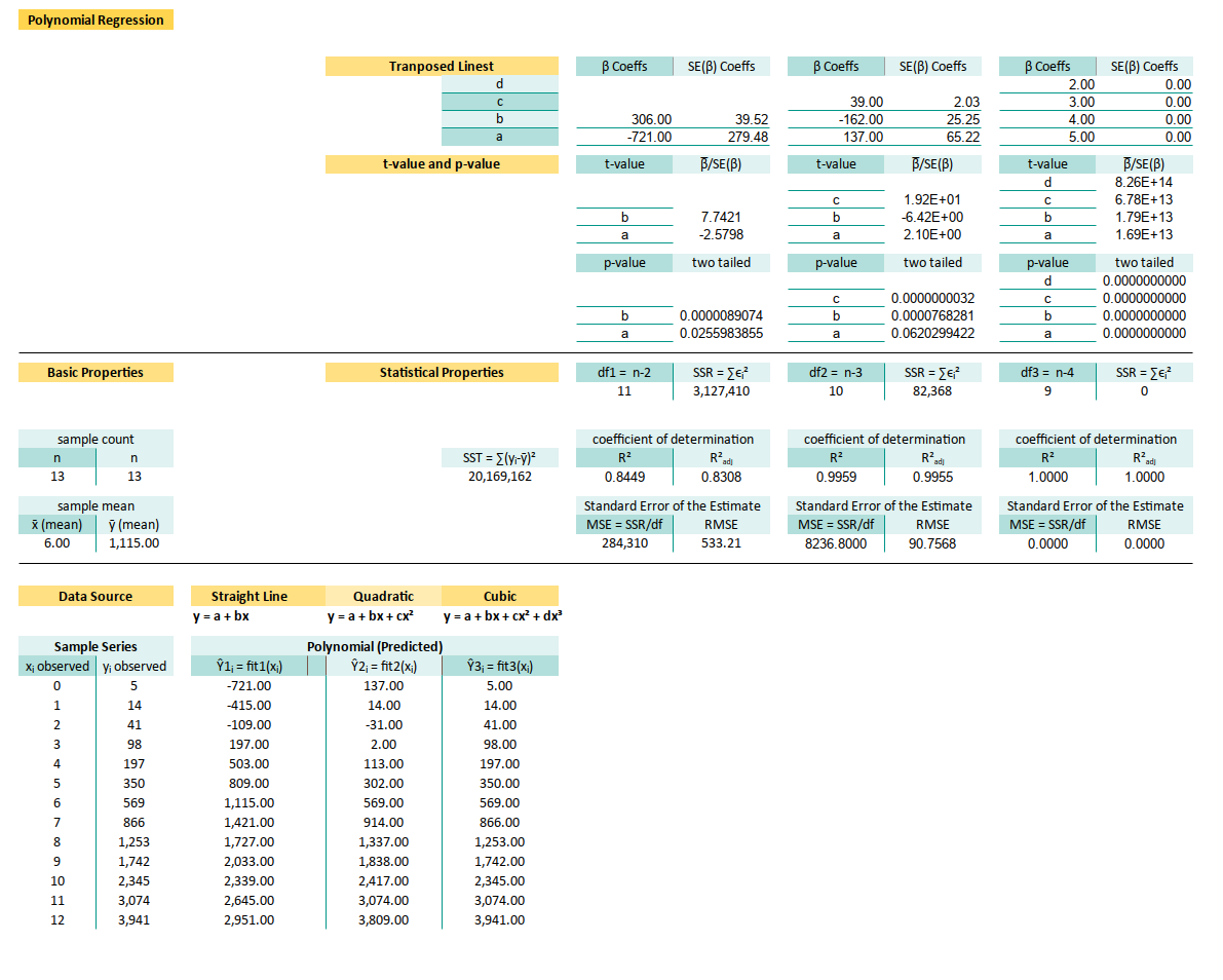
Complete Worksheet
Although this looks complex. It is easy when you have a working example. Here’s what the whole thing looks like, when it’s dressed up and ready for analysis:
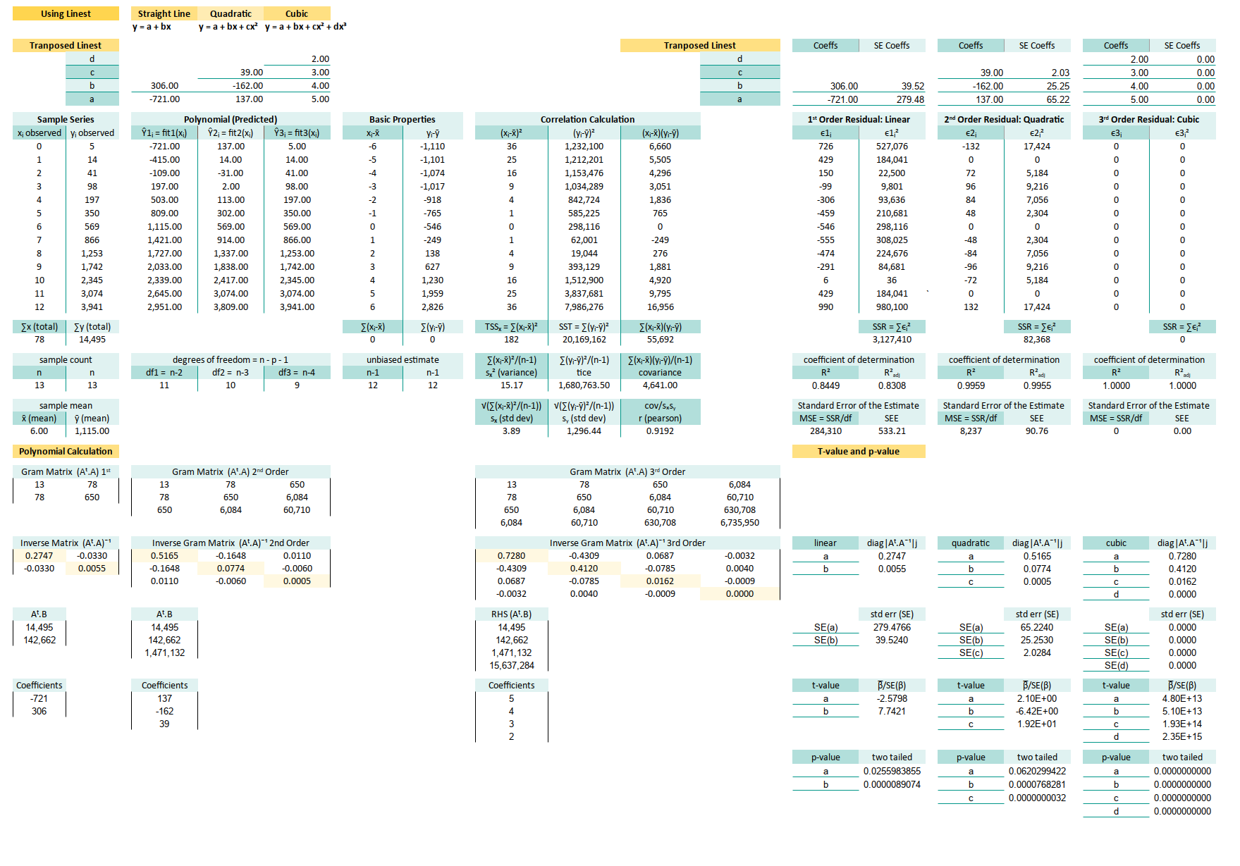
Yes, it’s long. Yes, it includes regression metrics, correlation, and some bonus bits. But it’s also user-friendly. We just input our observed values, and voilà—results.
The hardest part? Making complex things beginner-friendly without dumbing them down. That’s the magic trick here. We don’t need to understand all the backend sorcery, but it’s there when we’re curious.
We’ll walk through the core components in this article, using manual calculations. So you can trust, verify, or even recreate the magic from scratch.
2: Prediction using Linest
How to Cheat Elegantly with Built-In Magic.
In statistics, as in life, if there’s a shortcut that works. Take it, and pretend it was your plan all along!
The easiest way to perform polynomial regression in a spreadsheet? Just use LINEST.
Why reinvent the wheel when Excel already gave us a Formula-Ferrari?
Getting Coefficients
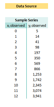
Let’s say our data lives in cells B13:C25,
where each (xᵢ, yᵢ) pair hangs out politely.
Here’s how to extract the polynomial coefficients using LINEST:
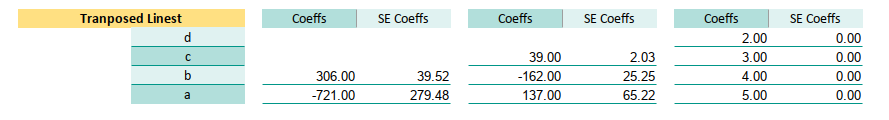
Linear: Range E8:E9
(=TRANSPOSE(LINEST(C13:C25,B13:B25)))

Quadratic: Range F7:F9
{=TRANSPOSE(LINEST(C13:C25,B13:B25^{1,2}))}

Cubic: Range: G6:G9
{=TRANSPOSE(LINEST(C13:C25,B13:B25^{1,2,3}))}
Where
- Linear Fit = first order
- Quadratic Fit = second order
- Cubic Fit = third order
This is our go-to method for quick regression. Ideal for most real-world use, especially when we’re prototyping, or need instant insights without full matrix rituals.
Getting Predictions
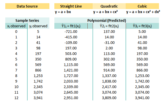
Now that you have our coefficients,
let’s put them to use and generate predicted values of Ŷᵢ = fit1(xᵢ) as:
And here’s how they look in Excel:
Linear: E13:E25
=$E$9+$E$8*B13

Quadratic: F13:F25
=$F$9+$F$8*B13+$F$7*B13^2

Cubic: G13:G25
=$G$9+$G$8*B13+$G$7*B13^2+$G$6*B13^3
These predictions let us model trends beyond straight lines. Ideal when our data clearly has curvature (and our boss clearly has expectations).
Done, without any complexity.
3: Prediction using Gram Matrix
How to Understand It Like a Real Nerd
What good is it learning without knowing how it works? Let’s go dive into the matrix.
Why use one function when you can suffer with 12?
The LINEST function is lovely,
until we want to understand what it’s actually doing.
Reverse engineer the calculation using manual calculation,
to understand how the math works internally.
Welcome to the Matrix 🧠. Here’s the classic normal equation in action:
We can compare the result to linest result directly.
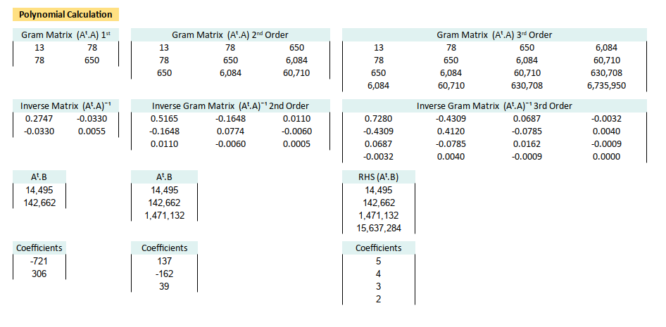
Gram Matrix (Aᵗ.A)
Now let’s break it into pieces using Excel formulas.
Linear: B42:C43
{=MMULT(
    TRANSPOSE(CHOOSE({1,2}, 1, B13:B25)),
    CHOOSE({1,2}, 1, B13:B25))}}

Quadratic: E42:G44
(=MMULT(
    TRANSPOSE(CHOOSE({1,2,3}, 1, B13:B25, B13:B25^2)),
    CHOOSE({1,2,3}, 1, B13:B25, B13:B25^2))))

Cubic: I42:L45
=MMULT(
    TRANSPOSE(CHOOSE({1,2,3,4}, 1, B13:B25, B13:B25^2, B13:B25^3)),
    CHOOSE({1,2,3,4}, 1, B13:B25, B13:B25^2, B13:B25^3))
This forms the core structure of our regression system. Like the chassis of a car, it doesn’t move on its own, but without it, we’re sitting on the road.
Inverse Gram Matrix (Aᵗ.A)ˉ¹
Linear: B48:C49
{=MINVERSE(B42:C43)}

Quadratic: E48:G50
{=MINVERSE(E42:G44)}

Cubic: I48:L51
{=MINVERSE(I42:L45)}
This lets us solve the system algebraically. Yes, crafting in Excel is slow, but we can now claim we “computed the inverse manually” at parties.
Right Hand Side (Aᵗ.B)
Linear: B54:B55
{=MMULT(
    TRANSPOSE(CHOOSE({1,2}, 1, B13:B25)),
    C13:C25)}}

Quadratic: E54:E56
{=MMULT(
    TRANSPOSE(CHOOSE({1,2,3}, 1, B13:B25, B13:B25^2)),
    C13:C25)}}

Cubic: I54:I57
{=MMULT(
    TRANSPOSE(CHOOSE({1,2,3,4}, 1, B13:B25, B13:B25^2, B13:B25^3)),
    C13:C25)}
This combines our design matrix with actual observed values i.e., this is where the “real world” enters our beautiful math.
Estimated Coefficients (β = [a, …])
Linear: B60:B61
{=MMULT(B48:C49,B54:B55)}

Quadratic: E60:E62
{=MMULT(E48:G50,E54:E56)}

Cubic: I60:I63
{=MMULT(I48:L51,I54:I57)}
We’ve reverse-engineered LINEST ,
nd proven to ourself that regression isn’t black magic.
Just highly organized matrix multiplication.
Yes, it’s a lot of formulas. But once we’ve wrangled Excel into solving matrix equations, we’ve basically earned your honorary statistician cape.
Using Raw Range Address
I keep the address cell, to keep basic spreadsheet, without named range feature that lead to incompatibility between different software.
If you think reading cell address is painful. I completely agree with you. Welcome to the club! In the next section, we’ll use named ranges to make things friendlier, more readable, and less like a crossword puzzle written by a matrix.
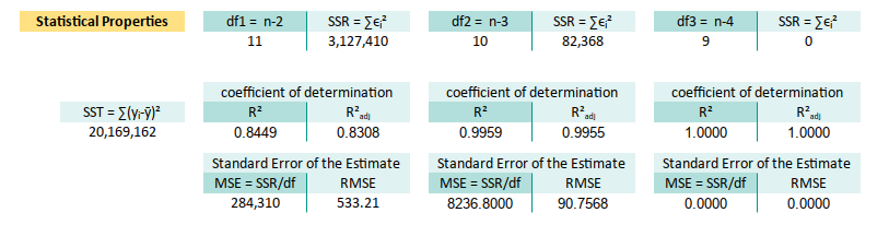
4: Degrees of Freedom
Freedom is not given, it is calculated.
Degrees of freedom (df) might sound like something philosophers argue over, but in regression, it’s just a headcount. How many data points we have minus how many coefficients we’re estimating (including the intercept). It tells us how much “wiggle room”, our model has before it starts overfitting like an overzealous intern.
The calculation of degree of freedom is obvious. I don’t think that It require detail descriptions.
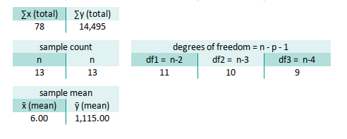
In our spreadsheet, that translates to:
Linear: E33
=COUNT($B$13:$B$25)-2

Quadratic: F33
=COUNT($B$13:$B$25)-3

Cubic: G33
=COUNT($B$13:$B$25)-4
Degrees of freedom influence standard errors, confidence intervals, and ultimately how much we can trust your model. No freedom = no fun = no inference.
5: Linear Properties
Correlation Calculation
“All models are wrong, but some have correlation.” – G.E.P. Box (probably)
We do not need all the basic correlaton properties here. We’re not chasing every detail of correlation properties here, just the essentials. Think of it like carrying only whatwe need for a hike: water, snacks, and maybe a chi-square joke.
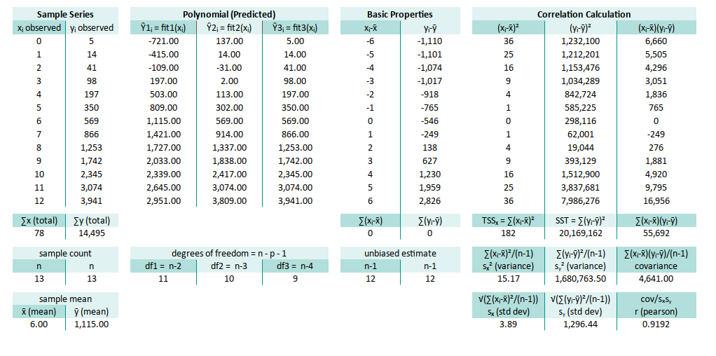
The variance, covariance and standard deviation here only applied to linear regression.
But however we still need this one thing: SST = ∑(yᵢ-ȳ)².
Here, we zoom in on the Total Sum of Squares (SST),
the granddaddy of variance in our model:
∑(yᵢ-ȳ)²: M28
=SUM(M13:M25)
This SST value tells us how much total variation is in our data. Later, we’ll see how much of that variation our model actually explains. The birth of R².
We don’t need anything else. Feel free to delete those unused variance/covariance cells, and then see what’s happened. Enjoy the slight thrill of living on the edge.
6: Standard Error using Linest
LINESTnot only draws the line, it confesses its uncertainty.
The LINEST function isn’t just a pretty face that spits out coefficients.
If we add the right optional arguments, it also gives us the standard errors,
which are basically the confidence level of each estimated β.
Think of them as the margin of error in our model’s smooth-talking predictions.
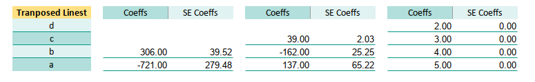
Getting Coefficients
Given our observed data pair (xᵢ, yᵢ) in B13:C25,
here’s how we summon both the coefficients,
and their standard errors, all in one go:
Linear: Range Q8:R9
=TRANSPOSE(LINEST(C13:C25,B13:B25,1,1))

Quadratic: Range T7:U9
=TRANSPOSE(LINEST(C13:C25,B13:B25^{1,2},1,1))

Cubic: Range: W6:X9
=TRANSPOSE(LINEST(C13:C25,B13:B25^{1,2,3},1,1))
With transpose, the standard error of the coefficients, is available in the second column. Now inn these ranges:
- First column: the coefficients (βs)
- Second column: the standard errors (how nervous each β is about its own value)
Standard error helps us judge which coefficients are pulling their weight, and which ones are just adding drama. A large standard error? That β might be bluffing.
7: Residual Properties
If it fits too well, it might be suspicious.
While LINEST generously hands us standard errors on a silver platter,
sometimes it’s good for the soul (and the brain) to cook the meal ourself.
By calculating residuals manually, we get to peek under the hood,
and understand how the standard error stew is really made.
Tabular Residual and SSR
Let’s roll up our sleeves and tabulate the residuals (ϵᵢ), their squares (ϵᵢ²), and also (∑ϵᵢ²) aka the sum of them all (SSE). This is the part where we count how much our model missed.
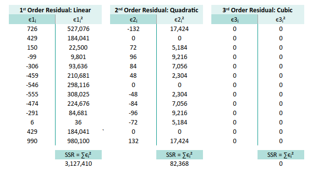
Remember the fit range? This is the address of predicted values for each model.
Y Observed: C13:C25
Linear: E13:E25
Quadratic: F13:F25
Cubic: G13:G25
Then we can compute residuals, like a true spreadsheet warrior, using the following formulas:
Linear:
* ϵᵢ   =$C13-E13
* ϵᵢ²  =Q13^2
* ∑ϵᵢ² =SUM(R13:R25) at R28

Quadratic:
* ϵᵢ   =$C13-F13
* ϵᵢ²  =T13^2
* ∑ϵᵢ² =SUM(U13:U25) at U28

Cubic:
* ϵᵢ   =$C13-G13
* ϵᵢ²  =W13^2
* ∑ϵᵢ² =SUM(X13:X25) at X28
The residuals are the noise our model failed to capture. Their sum of squares (SSE) tells us how far off our predictions are from the real world. The smaller, the better, unless we’re fitting noise instead of data.
Coefficient of Determination
Once we have SSE, we can compute the famous R². It’s the applause meter for our model, how much of the variance in our data is actually being explained. Now we can continue with R² and R²adjusted:
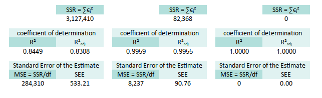
∑(yᵢ-ȳ)² at M28
df linear at E32
df quadratic at F32
df cubic at G32
Now plug ‘n play. We can substitute the formula.
Linear:
* R² =1-($R$28/$M$28) at Q32
* R²adjusted =1-((1-Q32)*($B$32-1)/$E32)

Quadratic:
* R² =1-($U$28/$M$28) at T32
* R²adjusted =1-((1-T32)*($B$32-1)/$E32)

Cubic:
* R² =1-($X$28/$M$28) at W32
* R²adjusted =1-((1-W32)*($B$32-1)/$E32)
R² tells us what portion of the chaos (variance) our model can explain. Adjusted R² keeps us honest, penalizing us for adding variables, that don’t pull their weight.
Standard Error of the Estimate
We now calculate the MSE (Mean Squared Error), and take its square root to get the SEE (Standard Error of the Estimate). Think of SEE as how far, on average, our predictions land from the truth. Kind of like our personal modeling credibility index.
With the same reference we can substitute MSE and SSE:
Linear:
* MSE =R28/$E$32 at Q36
* SEE =SQRT(Q36)

Quadratic:
* MSE =U28/$F$32 at T36
* SEE =SQRT(T36)

Cubic:
* MSE =X28/$G$32 at W36
* SEE =SQRT(W36)
SEE is your model’s average prediction error. If it’s too high, our model may need a tuning, or therapy.
Statiscian Joke
We have SEE, why can’t we have HEAR, or even SPEAK?
- We have
SEE(Standard Error of the Estimate), - but no
HEAR, because residuals never listen. - And certainly no
SPEAK, because p-values only whisper.
We are done.
8: Standard Error using Diagonal Matrix
Let’s revisit our beloved matrix form. This time, pay attention to the diagonals. They hold secrets. Specifically, the diagonals of the inverse Gram matrix are, proportional to the variances of the estimated coefficients.
The diagonal of inverse of gram matrix is actualy, the variance of the estimated coefficients, but required to be scaled.
The easiest thing to do is by pointing the cell,
for example Var(β₀) for linear fit is =B47.
But if we want to be looks like a real intellectual doing practical solution,
we can make ourself suffer using INDEX formula.
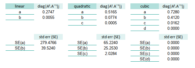
For example this tabulation of variance before scaled shown below. This is using alphabet notation (instead of beta):
Linear:
* a =INDEX(B47:C48,1,1)
* b =INDEX(B47:C48,2,2)

Quadratic:
* a =INDEX(E47:G49,1,1)
* b =INDEX(E47:G49,2,2)
* c =INDEX(E47:G49,3,3)

Cubic:
* a =INDEX(L47:O50,1,1)
* b =INDEX(L47:O50,2,2)
* c =INDEX(L47:O50,3,3)
* d =INDEX(L47:O50,4,4)
Now we can calculate the standard error by square root all of them.
Linear:
* SE(a) =SQRT($Q$36*R47)
* SE(b) =SQRT($Q$36*R48)

Quadratic:
* SE(a) =SQRT($T$36*U47)
* SE(b) =SQRT($T$36*U48)
* SE(c) =SQRT($T$36*U49)`

Cubic:
* SE(a) =SQRT($W$36*X47)
* SE(b) =SQRT($W$36*X48)
* SE(c) =SQRT($W$36*X49)
* SE(d) =SQRT($W$36*X50)
These standard errors tell us how stable our coefficients are. Large SE means that β might be throwing darts. Small SE? Now we’re talking precision.
That’s it. We’re al most finished.
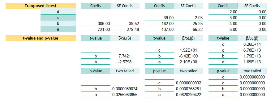
9: t-value and p-value
We’ve estimated the coefficients. We’ve calculated their standard errors. Now it’s time to interrogate them, are they just innocent bystanders, or guilty of being statistically significant?
Enter the t-value, our test statistic, the lie detector of linear modeling: by substituting the result of each SE(β).
The t-value tells us whether each coefficient is distinct from zero,
or just pretending to do something useful.
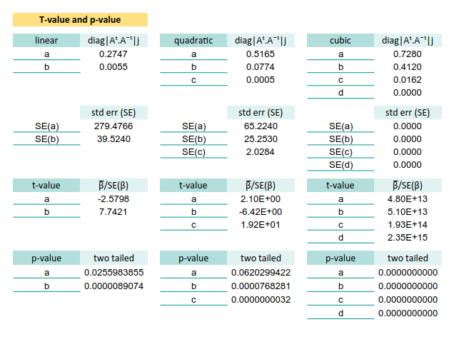
For example t-value in these cells below.
Let’s plug in the formulas and see who’s guilty.
Linear:
* t-value(a) =B59/R53
* t-value(b) =B60/R54

Quadratic:
* t-value(a) =B60/R54
* t-value(b) =E60/U54
* t-value(c) =E61/U55

Cubic:
* t-value(a) =L59/X53
* t-value(b) =L60/X54
* t-value(c) =L61/X55
* t-value(d) =L62/X56
Now, to determine just how guilty, we convert the t-values into p-values.
Think of this as how much evidence we have to doubt the null hypothesis.
Use T.DIST.2T (two-tailed test, because we’re equal opportunity skeptics):
Since we are using two tail, we are need ABS formula to avoid negative value.
Linear:
* p-value(a) =T.DIST.2T(ABS(R59),$E$32)
* p-value(b) =T.DIST.2T(ABS(R60),$E$32)

Quadratic:
* p-value(a) =T.DIST.2T(ABS(U59),$F$32)
* p-value(b) =T.DIST.2T(ABS(U60),$F$32)`
* p-value(c) =T.DIST.2T(ABS(U61),$F$32)

Cubic:
* p-value(a) =T.DIST.2T(ABS(X59),$G$32)`
* p-value(b) =T.DIST.2T(ABS(X60),$G$32)
* p-value(c) =T.DIST.2T(ABS(X61),$G$32)
* p-value(d) =T.DIST.2T(ABS(X62),$G$32)
Why the ABS()?
Because for two tailed, we don’t care which side the coefficient lies on.
If it’s far from zero, it better have a reason.
Tools Differences
Heads-up for tool differences. Libreoffice Calc and Excel might calculate inifinte number differently.
- Excel may yell
DIV/0!if a coefficient is completely flatlined. - LibreOffice is a bit more philosophical. it simply whispers 0 as if to say, “I saw nothing.”
Statistical detectives, we’ve done well. But alas, this sheet is way too long for daily patrol duty. Let’s prepare something shorter, sleeker, and more street-ready for practical regression analysis. Ready for that?
10: Practical Sheet
In real world daily basis, we should avoid the complexity.
Let’s face it, statistical elegance is nice, but when the boss says, “I want that trend report by lunch,”, we don’t have time to wrestle matrix algebra. We need a practical sheet. Something less like a math journal and more like a spreadsheet that doesn’t bite.
Data Entry Consideration
A key design principle of this worksheet: make data entry so easy our cat could do it. Real-world data isn’t always polite. It grows unpredictably. We might have 12 rows today and 120 tomorrow.
So, we let the data flow from the bottom up, like hot coffee in a cold mug. Statistical summaries stay at the top (where they don’t scroll away), while the raw data expands downward, like a rebellious teenager’s laundry pile.
Worksheet Source
Open-Source Fun, No Fine Print
This isn’t a proprietary black box. This is an artefact, baby. With named ranges and clean formulas, you can fork it, tweak it, break it, fix it, trash it, change it… (🎵 Daft Punk intensifies).
🧪 Get the sheet: github.com/…/math/trend/poly-regs.ods
You can open this document in LibreOffice.
LibreOffice recommended.
Because .ods is the new .xlsx.
The world is shifting.
Modern world needs modern tools.
ods is my choice.
Named Range
Named ranges are the breadcrumb trails for grown-up statisticians.
Rather than hunt for $O$6:$O$9, we call it coeff_3.
It’s like giving our matrix a proper name.
This is how the named range looks like in LibreOffice Calc. You can do the same thing with Microsoft Excel. But there are incompatibilies. Since I use LibreOffice for daily basis, This is what I’ve got.
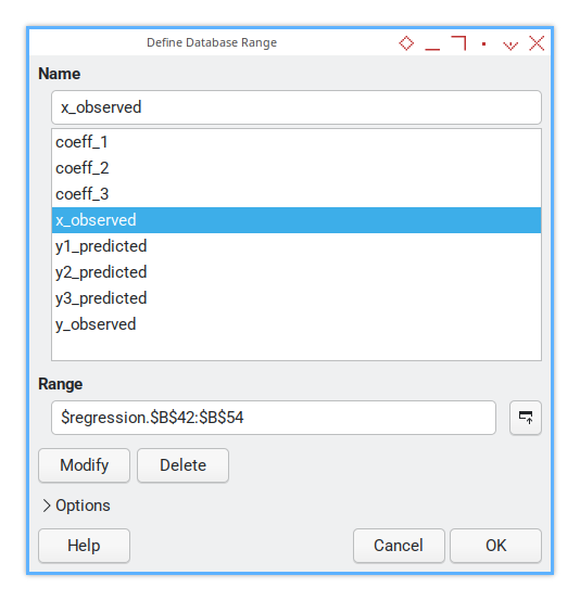
The steps are:
-
First I defined the observed range. From here I get the coefficient value (and standard error).
-
With coefficient value, I can calculate predicted values.
-
With predicted range I can calculate statistial properties.
Let say our sheet name is `regression’, Here’s how they’re laid out. The name address range can described as below:
| Named Range | Range Address |
|---|---|
| x_observed | $regression.$B$42:$B$54 |
| y_observed | $regression.$C$42:$C$54 |
| coeff_1 | $regression.$I$8:$I$9 |
| coeff_2 | $regression.$L$7:$L$9 |
| coeff_3 | $regression.$O$6:$O$9 |
| y1_predicted | $regression.$E$42:$E$54 |
| y2_predicted | $regression.$F$42:$F$54 |
| y3_predicted | $regression.$G$42:$G$54 |
Observed Value
Let’s start with observed value. The raw materials of our regression forge. The value might vary from samples to other samples, but let’s just use this example below:
Let’s set the named range with these cell address.
x_observed at B42:B54
y_observed at C42:C54“Garbage in, garbage out”, but here, we start with clean input.
Basic Properties
From this observed value we can calculate basic statistical properties. Before we fit fancy curves, let’s start with the humble mean.
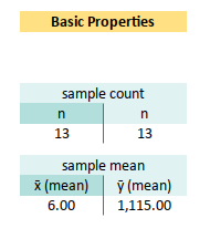
n =COUNT(x_observed) at B30
x̄ (mean) =AVERAGE(x_observed) at B34
ȳ (mean) =AVERAGE(y_observed) at C34
We use ȳ to calculate ∑(yᵢ-ȳ)². And we can completely dispose x̄ from the sheet. ȳ helps us measure how well our regression line explains the variance, and x̄… well, we don’t really use x̄ here.
Linest Result
Coefficient and Standard Error
The lazy genius method for coefficients and SE
Since we have already know how it works,
let Excel do the heavy lifting with LINEST.
Because life’s too short to invert a matrix manually.
| Name | Range |
|---|---|
| coeff_1 | $regression.$I$8:$I$9 |
| coeff_2 | $regression.$L$7:$L$9 |
| coeff_3 | $regression.$O$6:$O$9 |
Let’s choose that range, calculate, then set the named range with these cell address.
coeff_1 at I8:I9
=TRANSPOSE(LINEST(y_observed,x_observed,1,1))

coeff_2 at L7:L9
=TRANSPOSE(LINEST(y_observed,x_observed^{1,2},1,1))

coeff_3 at O8:O9
=TRANSPOSE(LINEST(y_observed,x_observed^{1,2,3},1,1))
It is more clear this way than using cell address right?
Saves time. Saves headaches.
In some countries, LINEST is prescribed as a stress reliever
Predicted Values
We plug our coefficients into the regression equation. Wwe can calculate the predicted values. But this time I’m going to use different formula, other than previously mentioned. This is our model speaking. I’ve seen the data, and here’s what I think.
y1_predicted at E42:E54
=SUMPRODUCT(TRANSPOSE(coeff_1),B43^{1,0})

y2_predicted at F42:F54
=SUMPRODUCT(TRANSPOSE(coeff_2),B43^{2,1,0})

y3_predicted at G42:G54
=SUMPRODUCT(TRANSPOSE(coeff_3),B43^{3,2,1,0})
Looks weird? It is even weirder when we understand that each coeff named range has two columns. Well.. Let’s get used to it.
t-value
We compute t-values to see if our coefficients,
are just making noise, or actually playing jazz.
t-value β₀ at K14
=J8/K8
We can just copy this cell to the rest of the t-value for each β.
It’s our detector.
-
A big
t-valuesays, “Hey, this coefficient might actually mean something.” -
A small one says, “Meh, maybe flip a coin.”
Degrees of Freedom
Freedom is beautiful.
Unless we subtract too many predictors.
In order to get the p-value, we need to calculate the degree of freedom.

Each polynomial degree costs us a degree of freedom.
Choose wisely, Padawan.
df1 at J25
=COUNT(x_observed)-2

df2 at M25
=COUNT(x_observed)-3

df3 at P25
=COUNT(x_observed)-4
Let’s compared with previous form.
Linear df: E33
=COUNT($B$13:$B$25)-2

Quadratic df: F33
=COUNT($B$13:$B$25)-3

Cubic df: G33
=COUNT($B$13:$B$25)-4
Now the formula would make sense right?
p-value
The p-value tells us how shocked you should be by the t-value.
Lower is better (unless you’re in an ethics committee).
t-value β₀ at K14
=J8/K8

p-value β₀
=T.DIST.2T(ABS(K14),$J$25)
We can just copy this cell to the rest of the p-value for each β.
It’s our detector.
- A small p-value? We’re probably on to something.
- A big one? Maybe it’s just statistical small talk.
Statistic Properties
We have different statistic properties, Let’s cover-up the formula one by one. This is the metrics that make or break our model’s ego.
SSR = ∑ϵᵢ²
Linear ∑ϵᵢ²: at K25
=SUMSQ(y_observed-y1_predicted)

Quadratic ∑ϵᵢ²: at M25
=SUMSQ(y_observed-y2_predicted)

Cubic ∑ϵᵢ²: at M25
=SUMSQ(y_observed-y3_predicted)
SST = ∑(yᵢ-ȳ)²
General:
ȳ (mean) at C34
=AVERAGE(y_observed)

SST = ∑(yᵢ-ȳ)² at H30
=SUMSQ(y_observed-$C$34)
R²
No improvement here. We go back to use address directly.
Linear R²: at J30
=1-($K$25/$H$30)

Quadratic R²: at M30
=1-($N$25/$H$30)

Cubic R²: at Q30
=1-($Q$25/$H$30)
MSE and RMSE
Linear:
MSE  =K25/$J$25 at J34
RMSE =SQRT(J34)

Quadratic:
MSE  =N25/$M$25 at M34
RMSE =SQRT(M34)

Cubic:
MSE  =Q25/$P$25 at Q34
RMSE =SQRT(P34)
And just like that, we’ve turned math into a working spreadsheet. Congratulations, we now speak fluent regressionese.
Next up? Let’s make this thing dance with charts.
What Lies Ahead 🤔?
So far, we’ve bravely navigated the polynomial seas , from linear models that behave to cubic ones that flirt with chaos. We’ve tamed the math, wrangled the formulas, and even convinced a spreadsheet to do our bidding (mostly without screaming). But what’s next?
We’re now shifting gears from “Why the math works”, to “How to actually use this without sacrificing our weekend.” Then let’s be honest: oour spreadsheet might be smart, ut it’s not going to code itself.
From Spreadsheet Zen to Python Wizardry 🐍✨
While a well-prepared spreadsheet can, make any office admin look like a statistical genius ("Oh this? It’s just my multi-degree polynomial model."), sometimes we need more power, flexibility, and sure fewer mouse clicks.
Spreadsheets are great for quick insights and small datasets, but when our data grows, or we want automation, reproducibility, or just prefer typing to dragging formulas with our mouse, Python becomes the natural habitat for our analytical side. Also, Python doesn’t forget our named ranges. Ever.
So what lies ahead?
- Practical code we can tweak, extend, or meme-ify.
- Visualizations to make sense of all these numbers.
- Tools to help us tell better data stories, or at least look cool while trying.
Let’s take the next step and walk into,
the land of pandas, numpy, and matplotlib with style.
You deserve it.
👉 Start here: [ Trend - Polynomial Regression - Python ].