Trend - Polynomial Regression - Theory

Preface

Goal: Goes further from linear regression to polynomial regression. The theoretical foundations, explains why the math works.

If linear regression is the “statistically safe” choice, like vanilla ice cream or using mean(), then polynomial regression is where things start getting fun. And slightly more dangerous.

The math gets spicy.

Polynomial regression isn’t just linear regression with more terms. Under the hood, it pulls in linear algebra concepts, like the Gram matrix, matrix transposes, and inverses. If these words sound intimidating, don’t worry. We will decode them one at a time.

⚠️ Warning: This article contains traces of matrix math. Those with linear algebra allergies should proceed with caution, or at least have a coffee in hand.

Cheatsheet

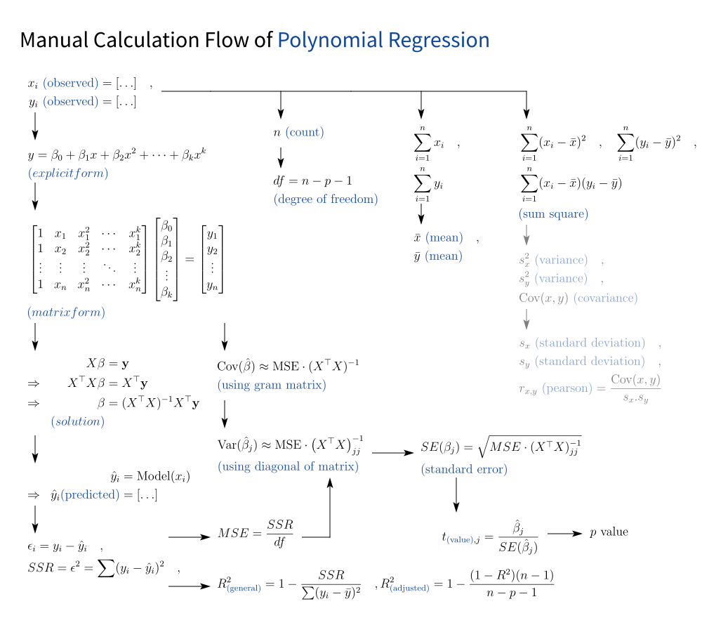
The Equation Flow

To help us navigate the swirling formulas, here’s a visual cheatsheet that ties everything together:

• The core regression model
• Error and residual breakdown
• Hypothesis testing logic
• And that sweet, sweet R² (plus the grown-up version: adjusted R²)

In one diagram, we will see how polynomial regression, gently parts ways from its linear sibling.

We can also grab the SVG version here (for printing, remixing, custom, black long sleeve t-shirt, or tattoo ideas):

📎 github.com/…/math/trend/equflow/equflow-04.svg

⚠️ A note for the statistically curious: This article only deals with samples, not populations. The math differs slightly, and yes, we’ll get to that later, still in this article.

Beyond This Basic

A must-have knowledge

With a solid grasp of polynomial regression, stepping into multivariate regression becomes much easier. Like swapping our socket wrench for a full torque-calibrated toolkit From here, we can smoothly move on to ANOVA, ANAREG, MANOVA, and beyond.

The underlying math principles stay familiar,. The workflows in spreadsheets is similar, We can build our own tabular data, just more columns to tune. Python stays approachable, still the same workbench. And PSPP? Built for everyday end-users like us, great for routine jobs.

In modern data science (DS), big data (BD), machine learning (ML), and AI, the real horsepower often comes from Bayesian Regression. Think of it as a royal marriage between two statistical dynasties: Regression and Probability.

To become a true AI engineer, we need to understand how both families work. Otherwise, we risk ending up as just a PyTorch/Keras/TensorFlow technician. Able to operate the tools, but not design the engine.

We will continue that journey, after we finish the Probability article series.

Basic Instinct

Years as engineering student, two decades, ago taught me the instinct to:

• Understand systems,
• Break down complexity,
• Explain it like it’s no big deal (in this blog or telegram),
• And when the system fails, not panic, but fix the blueprint.

So let’s start with blueprint.

---

1: Theoretical Backbone

Fitting Curves Without Losing Our Minds

Instead of focusing on Covariance, the equation is started with gram matrix.

This is the Equation for Polynomial Regression, but not the least square method. This is where we take raw data, and try to make it sing with the help of polynomials. Like karaoke, but with more math and less embarrassment.

Big Picture

Most of the equation in the left side part has been covered in polynomial calculation article.

• Trend - Polynomial Algebra

If you’ve already peeked at above algebra article, you have met most of these formulas before. No need for déjà vu. I don’t think that I need to refresh the equation over and over again. But let’s describe the equation notation in other forms.

Observed Data

We start with a humble set of observed data pairs:

$$\begin{align*} && {x_i}_\text{ (observed)} &= [\ldots] \quad , \\ && {y_i}_\text{ (observed)} &= [\ldots] \\ \end{align*}$$

Our mission (and we’ve chosen to accept it): find predicted values (by curve fittings).

$$\begin{align*} && {\hat{y}_i}_\text{ (prediction)} &= [\ldots] \\ \end{align*}$$

In essence, we want a curve that says: “I see your scatter, and I raise you a smooth function.”

Let’s find the solution for this using polynomial coefficients.

Fit Model

Polynomial Prediction Model

We have the generic theoritical model with this explicit form below. As cozy as a power series in a warm blanket.

$$y = \beta_0 + \beta_1 x + \beta_2 x^2 + \cdots + \beta_k x^k$$

But let’s keep things simple. Most of the time, we don’t go beyond cubic because:

• Linear (1st order):
  “Let’s just draw a line and see what happens.”

• Quadratic (2nd order):
  “Curvy, but still sober.”

• Cubic (3rd order):
  “Elegant, dramatic, but still behaves at dinner.”

$$\begin{array}{|l|l|l|} \hline \scriptstyle \text{1st order} & \scriptstyle \text{linear} & \hat{y}_i = \beta_0 + \beta_1{x_i} \rule{0pt}{2ex} \\ \hline \scriptstyle \text{2nd order} & \scriptstyle \text{quadratic} & \hat{y}_i = \beta_0 + \beta_1{x_i} + \beta_2{x_i}^2 \rule{0pt}{2ex} \\ \hline \scriptstyle \text{3rd order} & \scriptstyle \text{cubic} & \hat{y}_i = \beta_0 + \beta_1{x_i} + \beta_2{x_i}^2 + \beta_3{x_i}^3 \rule{0pt}{2ex} \\ \hline \end{array}$$

Where order is the degree of the polynomial. And β (beta) denotes the coefficients for specific polynomial degrees.

Higher-degree polynomials can capture more nuances (wiggles!), but beware the Curse of Overfitting™. Higher-order terms help model curvature, but also risk overfitting. This can be problematic in real world situations. Just because a model can hit every point doesn’t mean it should.

Matrix Form

Where Algebra Puts On Its Lab Coat

Enter the Vandermonde matrix, our handy companion for building polynomial models. In general this Vanderomonde is looks like this.

$$\begin{bmatrix} 1 & x_1 & x_1^2 & \cdots & x_1^k \\ 1 & x_2 & x_2^2 & \cdots & x_2^k \\ \vdots & \vdots & \vdots & \ddots & \vdots \\ 1 & x_n & x_n^2 & \cdots & x_n^k \\ \end{bmatrix} \begin{bmatrix} \beta_0 \\ \beta_1 \\ \beta_2 \\ \vdots \\ \beta_k \\ \end{bmatrix} = \begin{bmatrix} y_1 \\ y_2 \\ \vdots \\ y_n \\ \end{bmatrix} \\ $$

Where

• n: Number of observations (rows in X)

The Vandermonde matrix builds our X-values into powers, setting the stage for regression magic. The higher the column, the more wiggles our curve gets.

For the all three curve fittings, the actual matrix can be described as following:

$$\begin{array}{|l|l|l|} \hline \scriptstyle \text{linear} & \mathbf{X} = \begin{bmatrix} 1 & x_1 \\ 1 & x_2 \\ \vdots & \vdots \\ 1 & x_n \\ \end{bmatrix} & \mathbf{y} = \begin{bmatrix} y_1 \\ y_2 \\ \vdots \\ y_n \\ \end{bmatrix} \\ \hline \scriptstyle \text{quadratic} & \mathbf{X} = \begin{bmatrix} 1 & x_1 & x_1^2 \\ 1 & x_2 & x_2^2 \\ \vdots & \vdots & \vdots \\ 1 & x_n & x_n^2 \\ \end{bmatrix} & \mathbf{y} = \begin{bmatrix} y_1 \\ y_2 \\ \vdots \\ y_n \\ \end{bmatrix} \\ \hline \scriptstyle \text{cubic} & \mathbf{X} = \begin{bmatrix} 1 & x_1 & x_1^2 & x_1^3 \\ 1 & x_2 & x_2^2 & x_2^3 \\ \vdots & \vdots & \vdots & \vdots \\ 1 & x_n & x_n^2 & x_n^3 \\ \end{bmatrix} & \mathbf{y} = \begin{bmatrix} y_1 \\ y_2 \\ \vdots \\ y_n \\ \end{bmatrix} \\ \hline \end{array}$$

Solution

The Gram Matrix Moves In

It’s time for the main event: solving for the betas. The regression solution dances in with the Gram Matrix.

This is the solution, where X is the predictor variables, and y is dependent variables.

$$\begin{aligned} && X \mathbf{\beta} &= \mathbf{y} \\ \Rightarrow && X^\top X \mathbf{\beta} &= X^\top \mathbf{y} \\ \Rightarrow && \mathbf{\beta} &= (X^\top X)^{-1} X^\top \mathbf{y} \end{aligned}$$

This equation finds the best-fit coefficients, by minimizing the squared errors. Think of it as the least regret path, a statistically polite guess.

For each curve fittings, the coefficients solutions can be described as following:

$$\begin{array}{|l|l|} \hline \scriptstyle \text{linear} & \left(\mathbf{X}^T \mathbf{X}\right) \begin{bmatrix} \beta_0 \\ \beta_1 \\ \end{bmatrix} = \mathbf{X}^T \mathbf{y} \\ \hline \scriptstyle \text{quadratic} & \left(\mathbf{X}^T \mathbf{X}\right) \begin{bmatrix} \beta_0 \\ \beta_1 \\ \beta_2 \\ \end{bmatrix} = \mathbf{X}^T \mathbf{y} \\ \hline \scriptstyle \text{cubic} & \left(\mathbf{X}^T \mathbf{X}\right) \begin{bmatrix} \beta_0 \\ \beta_1 \\ \beta_2 \\ \beta_3 \\ \end{bmatrix} = \mathbf{X}^T \mathbf{y} \\ \hline \end{array}$$

Explicit Gram Matrix

Polynomial Symmetry Society

Now we also the generalized form the gram matrix (Xᵗ.X).

$$X^\top X = \begin{bmatrix} n & \sum x_m & \sum x_m^2 & \cdots & \sum x_m^k \\ \sum x_m & \sum x_m^2 & \sum x_m^3 & \cdots & \sum x_m^{k+1} \\ \sum x_m^2 & \sum x_m^3 & \sum x_m^4 & \cdots & \sum x_m^{k+2} \\ \vdots & \vdots & \vdots & \ddots & \vdots \\ \sum x_m^k & \sum x_m^{k+1} & \sum x_m^{k+2} & \cdots & \sum x_m^{2k} \end{bmatrix}$$

Where

• m: Index used in sums for (Xᵗ.X) entries

The Gram matrix is always symmetric, always serious.

We are going use computation. But for clarity, we can show the actual gram matrix for each curve fittings can be described as following:

$$\begin{array}{|l|l|} \hline \scriptstyle \text{linear} & \begin{bmatrix} n & \sum x_i \\ \sum x_i & \sum x_i^2 \\ \end{bmatrix} \begin{bmatrix} a \\ b \\ \end{bmatrix} = \begin{bmatrix} \sum y_i \\ \sum x_i y_i \\ \end{bmatrix} \\ \hline \scriptstyle \text{quadratic} & \begin{bmatrix} n & \sum x_i & \sum x_i^2 \\ \sum x_i & \sum x_i^2 & \sum x_i^3 \\ \sum x_i^2 & \sum x_i^3 & \sum x_i^4 \\ \end{bmatrix} \begin{bmatrix} a \\ b \\ c \\ \end{bmatrix} = \begin{bmatrix} \sum y_i \\ \sum x_i y_i \\ \sum x_i^2 y_i \\ \end{bmatrix} \\ \hline \scriptstyle \text{cubic} & \begin{bmatrix} n & \sum x_i & \sum x_i^2 & \sum x_i^3 \\ \sum x_i & \sum x_i^2 & \sum x_i^3 & \sum x_i^4 \\ \sum x_i^2 & \sum x_i^3 & \sum x_i^4 & \sum x_i^5 \\ \sum x_i^3 & \sum x_i^4 & \sum x_i^5 & \sum x_i^6 \\ \end{bmatrix} \begin{bmatrix} a \\ b \\ c \\ d \\ \end{bmatrix} = \begin{bmatrix} \sum y_i \\ \sum x_i y_i \\ \sum x_i^2 y_i \\ \sum x_i^3 y_i \\ \end{bmatrix} \\ \hline \end{array}$$

This matrix captures the relationship between predictor powers. Its symmetry is a mathematical peace treaty.

Inverse Gram Matrix

Matrix Gymnastics (Use Excel, Not Chalk)

To calculate each Coefficients, we need the inverse Gram Matrix (Xᵗ.X)ˉ¹ from the x observed values. There is no simple closed-form expression for inverse gram matrix (Xᵗ.X)ˉ¹. No need to brute-force the inverse by hand, just let Excel (or numpy) do the matrix gymnastics.

Fit Prediction

Prediction Time: Coefficients Meet X

Now that we have our shiny new estimated coefficients β (calculated from data), we plug them into our model and let the predictions flow.

$$\hat{\beta} = (X^\top X)^{-1} X^\top \mathbf{y}$$

Each xᵢ​ becomes the input to our polynomial machine.

Predicted Values

How Each Fit Performs, By Model Type

Using the estimated coefficients β, we substitute into the explicit polynomial forms. For each observed value xᵢ, we compute predictions yᵢ for each model:

$$\begin{array}{|l|l|} \hline \scriptstyle \textbf{Model Type} & \textbf{Prediction Equation} \\ \hline \scriptstyle \text{Observed predictors} & \mathbf{x} = [x_1, x_2, \ldots, x_n]^\top \\ \hline \scriptstyle \text{Linear fit} & \hat{y}_i = \hat{\beta}_0 + \hat{\beta}_1 x_i \\ \hline \scriptstyle \text{Quadratic fit} & \hat{y}_i = \hat{\beta}_0 + \hat{\beta}_1 x_i + \hat{\beta}_2 x_i^2 \\ \hline \scriptstyle \text{Cubic fit} & \hat{y}_i = \hat{\beta}_0 + \hat{\beta}_1 x_i + \hat{\beta}_2 x_i^2 + \hat{\beta}_3 x_i^3 \\ \hline \end{array}$$

Testing predictions against the observed values shows us, if the model is hugging the data… or ghosting it

Direct Comparison

Predicted vs Observed Values

The actual calculations use the same observed xᵢ values, enabling direct comparison with observed yᵢ. Compare these values side-by-side, and see how well our model hugs the data points:

$$\begin{array}{|l|l|} \hline \scriptstyle \text{samples} & {x_i}_\text{ (observed)} = [\ldots] \\ \hline \scriptstyle \text{samples} & {y_i}_\text{ (observed)} = [\ldots] \\ \hline \scriptstyle \text{linear} & {\hat{y}_i}_\text{ (prediction)} = [\ldots] \\ \hline \scriptstyle \text{quadratic} & {\hat{y}_i}_\text{ (prediction)} = [\ldots] \\ \hline \scriptstyle \text{cubic} & {\hat{y}_i}_\text{ (prediction)} = [\ldots] \\ \hline \end{array}$$

The model comparison reveals how polynomial complexity affects fit quality.

$$\begin{array}{|l|l|l|} \hline \text{Sample} & x_i \text{ (observed)} & y_i \text{ (observed)} \\ \hline 1 & x_1 & y_1 \\ 2 & x_2 & y_2 \\ \vdots & \vdots & \vdots \\ n & x_n & y_n \\ \hline \end{array}$$ $$\begin{array}{|l|l|l|l|} \hline \text{Prediction} & \text{Linear} & \text{Quadratic} & \text{Cubic} \\ \hline \hat{y}_1 & \hat{\beta}_0 + \hat{\beta}_1 x_1 & \hat{\beta}_0 + \hat{\beta}_1 x_1 + \hat{\beta}_2 x_1^2 & \hat{\beta}_0 + \cdots + \hat{\beta}_3 x_1^3 \\ \hat{y}_2 & \hat{\beta}_0 + \hat{\beta}_1 x_2 & \hat{\beta}_0 + \hat{\beta}_1 x_2 + \hat{\beta}_2 x_2^2 & \hat{\beta}_0 + \cdots + \hat{\beta}_3 x_2^3 \\ \vdots & \vdots & \vdots & \vdots \\ \hat{y}_n & \hat{\beta}_0 + \hat{\beta}_1 x_n & \hat{\beta}_0 + \hat{\beta}_1 x_n + \hat{\beta}_2 x_n^2 & \hat{\beta}_0 + \cdots + \hat{\beta}_3 x_n^3 \\ \hline \end{array}$$

Seeing how predictions match the actual data helps us choose the right model. It’s like a job interview for polynomials.

Only the best fit gets hired.

The interesting parts comes in the next section below.

---

2: Equation for Regression

When linear thinking just doesn’t cut it.

Polynomial regression doesn’t just bend the line. It bends our brain a little too. The equations look familiar… until they don’t.

Cheat mode reminder: Many formulas here were foreshadowed in

• Trend - Properties - Cheatsheet

This section walks through the theory with a gentle curve (pun intended), showing what’s really happening under the Excel hood or Python matrix.

No Variance?

Where’s the Usual Gang?

Where’s Standard Deviation? Where’s Waldo? Where’s my sanity?

In linear regression, we hang out with slope, intercept, Pearson’s r, and the rest of the cool kids. But in polynomial regression? Some of those buddies don’t get invited.

• Standard deviation? Only for total variance, not slope.
• Covariance? Still around, but much sneakier.
• Intercept and slope? Replaced with a full orchestra of betas.

So where is the famous Standard Deviation? Pearson, and covariance? Actually these properties are only relevant for linear regression.

Still, we calculate total variance (SST) the same way, with mean inside the equation.

$$\sum (y_i - \bar{y})^2$$

This total variance is our baseline. The “total noise” we’re trying to explain with our curve. Even if the curve squiggles, the goal remains: reduce this total chaos.

We still have covariance, but not in the simple form as used in previous linear regression.

Degrees of Freedom

More predictors = more complexity = fewer degrees of freedom.

It’s like giving a child too many crayons. Things get wilder, but less meaningful.

In polynomial regression, the degrees of freedom (df) for the error term (residuals) is calculated as:

$$\begin{align*} & df = n - p - 1 \\ & \scriptstyle \text{(degree of freedom)} \end{align*}$$

Where the equation itself can be interpreted as:

• n = Total number of observations (data points).
• p = Number of predictors (independent variables) in the model.
• -1 = Accounts for the intercept term (β₀​).

The use of the predictors is pretty clear for each case. Now we can rewrite for each model as:

$$\begin{array}{|l|l|l|} \hline \scriptstyle \text{linear} & p = 1: \text{only } x & df = n - 2 \\ \hline \scriptstyle \text{quadratic} & p = 2: x \text{ and } x^2 & df = n - 3 \\ \hline \scriptstyle \text{cubic} & p = 3: x, x^2, x^3 & df = n - 4 \\ \hline \end{array}$$

df controls how “penalized” our model is for being fancy. Without it, we’d just keep adding powers of x until the model folds in on itself.

Residual

Where the Errors Hide

The SSE (Sum of Squared Errors) is still the champion of model diagnostics. SSE is calculated the same way for all models, but the residuals differ based on the model’s complexity:

$$\begin{align*} SSE &= \sum\limits_{i=1}^{n} (\epsilon_i)^2 \\ &= \sum (y_i - \hat{y}_i)^2 \\ \end{align*}$$

Where the predicted values of ŷᵢ vary by model. Each ŷᵢ​ is shaped by our model’s ego:

$$\begin{array}{|l|l|} \hline \scriptstyle \text{linear} & \sum (y_i - \left(\beta_0 + \beta_1{x_i})\right)^2 \\ \hline \scriptstyle \text{quadratic} & \sum (y_i - \left(\beta_0 + \beta_1{x_i} + \beta_2{x_i}^2)\right)^2 \\ \hline \scriptstyle \text{cubic} & \sum (y_i - \left(\beta_0 + \beta_1{x_i} + \beta_2{x_i}^2 + \beta_3{x_i}^3)\right)^2 \\ \hline \end{array}$$

Don’t worry, we are not going to derive these equation. We’ll compute these directly in Excel using tabular calculations.

Residuals are the leftover errors our model couldn’t explain. Polynomial regression lets our line dance more freely to reduce them. But it also risks overfitting the floor.

Coefficient of Determination

The R Square (R²), the ego meter of our model.

In general, the R Square (R²) is still defined as follows.

$$R^2 = 1 - \frac{\sum (y_i - \hat{y}_i)^2}{\sum (y_i - \bar{y})^2}$$

Using tabular in Excel (or python), we can just put the residual calculation above into above equation. Still works the same. Just plug in new predictions.

And here comes the wise sibling. We can calculate the adjusted R Square with following equation:

$$R^2 _\text{(adjusted)} = 1 - \frac{{(1 - R^2)(n - 1)}}{{n - p - 1}}$$

Adjusted R² keeps us honest. It says: “Sure, our curve fits well, but did it really earn it?”

MSE

The average shame of our models predictions.

MSE stand for Mean Standard Errors. The mean word refers to the average of squared errors, adjusted for degrees of freedom.

$$MSE = \frac{SSE}{df} = \frac{\sum (y_i - \hat{y}_i)^2 }{n - p - 1}$$

Then take the square root for Root Mean Squared Error (RMSE), as a helper for further calculation.

$$RMSE = \sqrt{MSE}$$

MSE is the backbone of every test and confidence interval that follows Think of it as our model’s humility score.

Gram Matrix

To calculate Standard Error of each Coefficients, we need Gram Matrix (Xᵗ.X) from the x observed values.

From the matrix form:

$$X = \begin{bmatrix} 1 & x_1 & x_1^2 & \cdots & x_1^k \\ 1 & x_2 & x_2^2 & \cdots & x_2^k \\ \vdots & \vdots & \vdots & \ddots & \vdots \\ 1 & x_n & x_n^2 & \cdots & x_n^k \\ \end{bmatrix}$$

This matrix is like our model’s blueprint. Without it, you can’t build standard errors, variances, or credibility.

Covariance Matrix of β

β = coefficient estimates

The theoretical covariance matrix is:

$$\text{Cov}(\hat{\mathbf{\beta}}) = \sigma^2 (X^\top X)^{-1}$$

where:

• σ² is the true error variance (unknown in practice)
• (Xᵗ.X)ˉ¹ is the inverse Gram matrix

In practice, we estimate σ² using the Mean Squared Error (MSE):

$$\text{Cov}(\hat{\mathbf{\beta}}) \approx \text{MSE} \cdot (X^\top X)^{-1}$$

To find inverse gram matrix (Xᵗ.X)ˉ¹, we have to rely on computation instead of finding generalization equation.

Variance of β

β = coefficient estimates

The true variance of the coefficient estimates is

$$\text{Var}(\hat{\beta}_j) = \sigma^2 \cdot \left(X^\top X\right)^{-1}_{jj}$$

Where

• σ² is the unknown error variance

In practice, we estimate σ² using the Mean Squared Error (MSE):

$$\text{Var}(\hat{\beta}_j) \approx \text{MSE} \cdot \left(X^\top X\right)^{-1}_{jj}$$

Want to know how “wobbly” each coefficient is? This tells us.

High variance = less trust.

Diagonal Matrix

The diagonal of the inverse Gram matrix, the diags|(Xᵗ.X)ˉ¹|, represents the scaled variance of β (variance per unit of σ²):

$$\left(X^\top X\right)^{-1}_{jj} \approx \text{Var}_{scaled}(\hat{\beta}_j)\cdot$$

Or in other notation can be written as

$$\text{diag}|(X^\top X)^{-1}|_j$$

The same applied for diags|(Xᵗ.X)ˉ¹|ⱼ. There is no generalization either, so we have to rely on computation instead.

No closed formula. Just crunch it.

Standard Error of Coefficient

Like standard deviation, but for the guesswork inyour βs.

Standard deviation is the square root of the variance right? Then the standard error (SE) is indeed, the square root of the variance of the coefficient estimates.

For any coefficient βⱼ​ in polynomial regression:

$$\begin{align*} SE(\hat{\beta}_j) &= \sqrt{\text{Var}(\hat{\beta}_j) } \\ &= \sqrt{MSE \cdot (X^\top X)^{-1}_{jj}} \end{align*}$$

We can break down for each case. The standard Errors by Polynomial Degree are:

$$\begin{array}{|l|l|} \hline \scriptstyle \text{linear} & SE(\hat{\beta}_0) , SE(\hat{\beta}_1) \\ \hline \scriptstyle \text{quadratic} & SE(\hat{\beta}_0) , SE(\hat{\beta}_1) , SE(\hat{\beta}_2) \\ \hline \scriptstyle \text{cubic} & SE(\hat{\beta}_0) , SE(\hat{\beta}_1) , SE(\hat{\beta}_2) , SE(\hat{\beta}_3) \\ \hline \end{array}$$

These errors define our confidence intervals, t-tests, and how much trust we place in each term.

A high SE(βⱼ)? Suspicious term (predictor like x² or x³) may not actually be contributing useful information to the model. It’s possibly just capturing random variation in the data (i.e., noise). In polynomial regression, as we add higher-degree terms, some of them might look like they fit better. But if their standard errors are large it’s a red flag.

t-value

In Polynomial Regression

Want to know if a coefficient is doing real work, or just lounging around?

The t-value for each coefficient β​ tests the null hypothesis H₀: βj=0. It is calculated as:

$$t_{\text{value}, j} = \frac{\hat{\beta}_j}{SE(\hat{\beta}_j)}$$

Where:

• Numerator β​ = Estimated coefficient
• Denumerator SE(β) = Standard error of β​ (from previous section)

H₀: βⱼ=0 asserts that the predictor xⱼ (e.g., x, x², etc.), has no effect on the response variable y. If H₀​ is true, the term xⱼ should be dropped from the model.

This is our litmus test. If βⱼ​ is tiny, maybe your precious x² or x³ isn’t adding value.

p-value

Just trust Excel or Python!

No need any gamma function complexity for practical calculation by hand. For beginner like us, it is better to use excel built-in fomula instead.

p-values tell us whether to keep or dump predictors. It’s like speed dating for variables.

Confidence Intervals

We can continue to other statistical properties beyond just coefficients. There’s more we could calculate: confidence bounds, prediction intervals, F-tests. But let’s save that for next time. I guess I need to stop before this article become to complex. Let’s keep this article to be statistics for beginner.

NNow’s the time to tabulate all of this in Excel, or code it in Python for style points. Just remember: under all these equations, we’re still doing one thing. Trying to explain variance without overfitting our sanity.

---

What Lies Ahead 🤔?

Math is fun, right?

No, really! Don’t run away just yet!

From theoretical foundations we are going shift to practical implementation in daily basis, using spreadsheet formula, python tools, and visualizations. Now that we’ve untangled the algebra spaghetti of polynomial regression, it’s time to roll up our sleeves and get our hands dirty, with Excel, Python, and a healthy skepticism of curve fitting gone wild.

While the theory explains why the math works, the practice shows how to execute it with real tools. With the flow, from theory to tabular spreadsheets, then from we are going to build visualization using python.

The theory gives us the why. Why these equations matter, why the degrees of freedom shrink, faster than our confidence in a stats exam, and why that suspicious x³ term might just be freeloading. But knowing isn’t enough. The real-world payoff comes in the how:

• How to implement all this using spreadsheet formulas (yes, even Excel deserves love)
• How to double-check our coefficients without crying into our coffee
• How to visualize trends like a pro using Python

We’re shifting gears: from theory to table, from formula to function, from blackboard to browser. Whether we’re working on trend analysis for stock prices, or just trying to figure out if our cat’s weight gain is linear or exponential (spoiler: it’s usually cubic around holidays), this next step matters.

Time to move from “hmm, interesting” to “aha!” Curious to see it all come together? March forward to 👉 [ Trend – Polynomial Regression – Formula ].