Preface
Goal: Getting to know statistical properties, using python library step by step.
Why are we even doing this?
We should know the statistical concept, before wrestling with a statistical model using worksheet formula. Understanding what the mean, variance, skewness, and their rowdy cousins really do helps us, in debugging more effectively, when something goes wrong in our calculation.
Here’s the usual path:
- Understand the equation.
- Implement it in a spreadsheet.
- Rebuild it in Python like a proper data monk.
- Use it for slick plots, automation, or feeding it into AI models.
We’re not just learning stats. We’re learning how to weaponize stats with tools like, pandas, numpy, and scipy. One property at a time.
From equation, and statistic model in worksheet. we can step further to implement the model in scripting. This way we can go further with automation, nice visualization, and combine with other technologies.
Manual Calculation
Doing it the hard way, so Python doesn’t have to.
Before we let libraries like scipy do all the heavy lifting, it’s important to know what they’re actually doing under the hood. Think of this as the “manual transmission” part of statistical driving. We’ll understand the gears better before hitting the cruise control.
We can summarize all manual calculation of, statistic properties from previous worksheet with python:
Python Source
All the Python sorcery we’re about to walk through lives here:
Data Source
We’ve moved past hardcoded numbers. Let’s be civilized and use a CSV:
What’s inside?
A sweet little dataset with x_observed and y_observed pairs.
x,y
0,5
1,12
2,25
3,44
4,69
5,100
6,137
7,180
8,229
9,284
10,345
11,412
12,485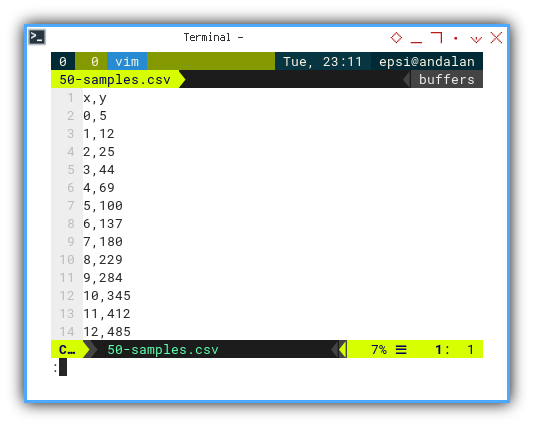
Loading Data Series
First, we politely invite the data into memory:
import numpy as np

# Getting Matrix Values
pairCSV = np.genfromtxt("50-samples.csv",
  skip_header=1, delimiter=",", dtype=float)

# Extract x and y values from CSV data
x_values = pairCSV[:, 0]
y_values = pairCSV[:, 1]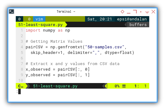
Garbage in, garbage out. Always know how our data is being loaded.
Basic Properties
Time to warm up with some classic stats:
# Number of data points
n = len(x_observed)

# Calculate sums
x_sum = np.sum(x_observed)
y_sum = np.sum(y_observed)

# Calculate means
x_mean = np.mean(x_observed)
y_mean = np.mean(y_observed)

# Output of basic properties
print(f'{f"n":10s} = {n:4d}')
print(f'∑x (total) = {x_sum:7.2f}')
print(f'∑y (total) = {y_sum:7.2f}')
print(f'x̄ (mean)   = {x_mean:7.2f}')
print(f'ȳ (mean)   = {y_mean:7.2f}')
print()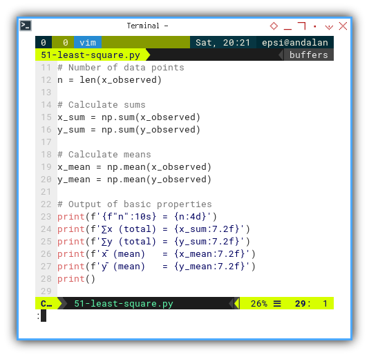
These are the building blocks. Like knowing the flour, sugar, and eggs before we bake a regression cake.
Deviations
Now we look at how each point misbehaves compared to the average. Deviations are the rebels of our dataset, with the least square coefficient:
# Calculate deviations
x_deviation = x_observed - x_mean
y_deviation = y_observed - y_mean

# Calculate squared deviations
x_sq_deviation = np.sum(x_deviation ** 2)
y_sq_deviation = np.sum(x_deviation ** 2)

# Calculate cross-deviation
xy_cross_deviation = np.sum(x_deviation * y_deviation)
# Calculate slope (m) and intercept (b)
m_slope = xy_cross_deviation / x_sq_deviation
b_intercept = y_mean - m_slope * x_mean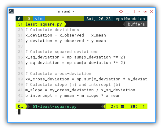
Now let’s print our slope-intercept poetry, in terminal.
# Output of least square calculation
print(f'∑(xᵢ-x̄)    = {np.sum(x_deviation):9.2f}')
print(f'∑(yᵢ-ȳ)    = {np.sum(y_deviation):9.2f}')
print(f'∑(xᵢ-x̄)²   = {x_sq_deviation:9.2f}')
print(f'∑(yᵢ-ȳ)²   = {y_sq_deviation:9.2f}')
print(f'∑(xᵢ-x̄)(yᵢ-ȳ)  = {xy_cross_deviation:9.2f}')
print(f'm (slope)      = {m_slope:9.2f}')
print(f'b (intercept)  = {b_intercept:9.2f}')
print()

print(f'Equation     y = ' \
  + f'{b_intercept:5.2f} + {m_slope:5.2f}.x')
print()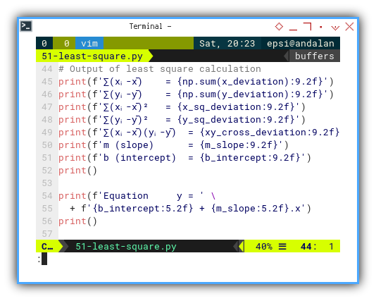
This is our regression line. If stats were a rom-com, this would be the love interest. Everything leads to this.
Variance and Covariance
Let’s dive into the spread of our data, and their relationship status by getting the R square:
# Calculate variance
x_variance = x_sq_deviation / n
y_variance = y_sq_deviation / n

# Calculate covariance
xy_covariance = xy_cross_deviation / n

# Calculate standard deviations
x_std_dev = np.sqrt(x_variance)
y_std_dev = np.sqrt(y_variance)

# Calculate Pearson correlation coefficient (r)
r = xy_covariance / (x_std_dev * y_std_dev)

# Calculate R-squared (R²)
r_squared = r ** 2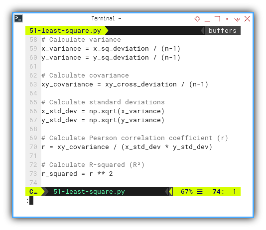
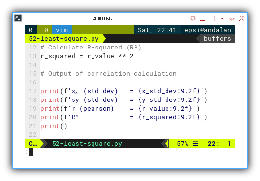
Print it loud and proud:
# Output of correlation calculation
print(f'sₓ² (variance) = {x_variance:9.2f}')
print(f'sy² (variance) = {y_variance:9.2f}')
print(f'covariance     = {xy_covariance:9.2f}')
print(f'sₓ (std dev)   = {x_std_dev:9.2f}')
print(f'sy (std dev)   = {y_std_dev:9.2f}')
print(f'r (pearson)    = {r:9.2f}')
print(f'R²             = {r_squared:9.2f}')
print()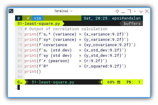
R² tells you how well our model is doing. If it’s close to 1, our model’s a genius. If not… maybe go meditate on your data.
Residuals
This is where we check how wrong we are, elegantly. Let’s get the correlation, until we get the t-value.
# Create regression line
y_fit = m_slope * x_observed + b_intercept
y_err = y_observed - y_fit

# Calculate sum of squared residuals
ss_residuals = np.sum(y_err ** 2)

# Calculate degrees of freedom
df = n - 2

# Calculate variance of residuals (MSE)
var_residuals = ss_residuals / df

# Calculate standard error of the slope
std_err_slope = np.sqrt(var_residuals / x_sq_deviation)

# Calculate t-value
t_value = m_slope / std_err_slope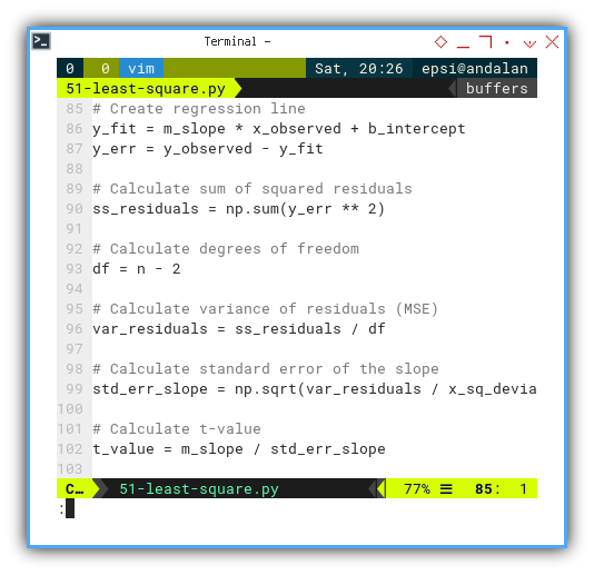
Wrap it up with a bow:
# Output the results
print(f'SSR = ∑ϵ²           = {ss_residuals:9.2f}')
print(f'MSE = ∑ϵ²/(n-2)     = {var_residuals:9.2f}')
print(f'SE(β₁)  = √(MSE/sₓ) = {std_err_slope:9.2f}')
print(f't-value = β̅₁/SE(β₁) = {t_value:9.2f}')
print()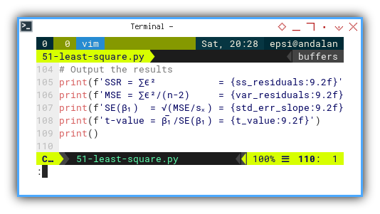
The t-value gives use an idea of how significant your slope is.
If it’s large, congratulations,
Our regression is statistically more than just a coincidence.
Output Result
Here’s the satisfying full output, no magic, no black boxes. Just raw, honest math:
n          =   13
∑x (total) =   78.00
∑y (total) = 2327.00
x̄ (mean)   =    6.00
ȳ (mean)   =  179.00

∑(xᵢ-x̄)    =      0.00
∑(yᵢ-ȳ)    =      0.00
∑(xᵢ-x̄)²   =    182.00
∑(yᵢ-ȳ)²   = 309218.00
∑(xᵢ-x̄)(yᵢ-ȳ)  =   7280.00
m (slope)      =     40.00
b (intercept)  =    -61.00

Equation     y = -61.00 + 40.00.x

sₓ² (variance) =     14.00
sy² (variance) =  23786.00
covariance     =    560.00
sₓ (std dev)   =      3.74
sy (std dev)   =    154.23
r (pearson)    =      0.97
R²             =      0.94

SSR = ∑ϵ²           =  18018.00
MSE = ∑ϵ²/(n-2)     =   1638.00
SE(β₁)  = √(MSE/sₓ) =      3.00
t-value = β̅₁/SE(β₁) =     13.33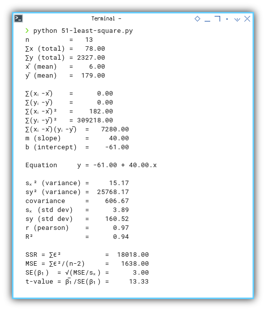
This is the full audit trail. If a fellow nerd asks, “Did you check the residuals?”, we can say “Absolutely.”
Interactive JupyterLab
Want to play with it live? Fire up the interactive version here:
You can obtain the interactive Jupyter Notebook in this following link:
Properties Helper
As you can see the the script above is too long, for just obtaining least square coefficient. We can simply use with python library, to get only what we need, then shorten the script.
We also need to refactor the code for reuse, So before that we need to solve this refactoring issue.
Handling Multiple Variables
Script above using a lot of statistics properties, these local variables are scattered, and the worst part is we don’t know what we need, while doing statistic exploration. This makes coding harder to modularized.
With python we can use python locals() built-in method.
With this locals(), we can bundle all variables as dictionary.
def get_properties(file_path) -> Dict:
  ...

  return locals()
The in other python files, we can load properties from `Properties.py`` helper and unpack them into local variables.
properties = get_properties("50-samples.csv")
locals().update(properties)
Now, in our other Python scripts, we can just call this like ordering takeout:
def display(properties: Dict) -> None:
  p = Dict2Obj(properties)

  ...
Or go full OOP and pass them around in a function:
class Dict2Obj:
  def __init__(self, properties_dict):
    self.__dict__.update(properties_dict)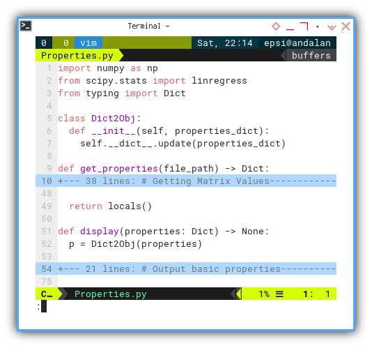
The Properties Helper
Let’s build a reusable Python helper for basic statistical properties. Think of this as our multipurpose wrench for trend analysis.
The helper has two main parts:
get_properties()for computationdisplay()for output
The first half is similar to our earlier longhand script. But now it’s organized and tucked inside a function:
def get_properties(file_path) -> Dict:
  # Getting Matrix Values
  pairCSV = np.genfromtxt(file_path,
    skip_header=1, delimiter=",", dtype=float)

  # Extract x and y values from CSV data
  x_observed = pairCSV[:, 0]
  y_observed = pairCSV[:, 1]

  # Number of data points
  n = len(x_observed)

  # Calculate sums
  x_sum = np.sum(x_observed)
  y_sum = np.sum(y_observed)

  # Calculate means
  x_mean = np.mean(x_observed)
  y_mean = np.mean(y_observed)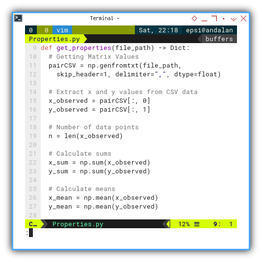
Now, let’s crank the gears using numpy:
  # Calculate variance
  x_variance = np.var(x_observed)
  y_variance = np.var(y_observed)

  # Calculate covariance
  xy_covariance = np.cov(x_observed, y_observed)[0, 1]

  # Calculate standard deviations
  x_std_dev = np.std(x_observed)
  y_std_dev = np.std(y_observed)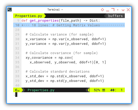
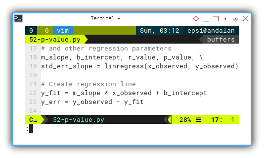
And then we can get the regression using linregress():
  # Calculate slope (m), intercept (b),
  # and other regression parameters
  m_slope, b_intercept, r_value, p_value, \
  std_err_slope = linregress(x_observed, y_observed)

  # Create regression line
  y_fit = m_slope * x_observed + b_intercept
  y_err = y_observed - y_fit

  return locals()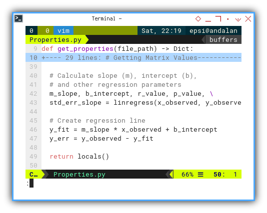
Then we can display the properties in different function. Separating the model and the view.
def display(properties: Dict) -> None:
  p = Dict2Obj(properties)

  # Output basic properties
  print(f'{f"n":10s} = {p.n:4d}')
  print(f'∑x (total) = {p.x_sum:7.2f}')
  print(f'∑y (total) = {p.y_sum:7.2f}')
  print(f'x̄ (mean)   = {p.x_mean:7.2f}')
  print(f'ȳ (mean)   = {p.y_mean:7.2f}')
  print()

  # Output statistics properties
  print(f'sₓ² (variance) = {p.x_variance:9.2f}')
  print(f'sy² (variance) = {p.y_variance:9.2f}')
  print(f'covariance     = {p.xy_covariance:9.2f}')
  print(f'sₓ (std dev)   = {p.x_std_dev:9.2f}')
  print(f'sy (std dev)   = {p.y_std_dev:9.2f}')
  print(f'm (slope)      = {p.m_slope:9.2f}')
  print(f'b (intercept)  = {p.b_intercept:9.2f}')
  print()

  print(f'Equation     y = ' \
    + f'{p.b_intercept:5.2f} + {p.m_slope:5.2f}.x')
  print()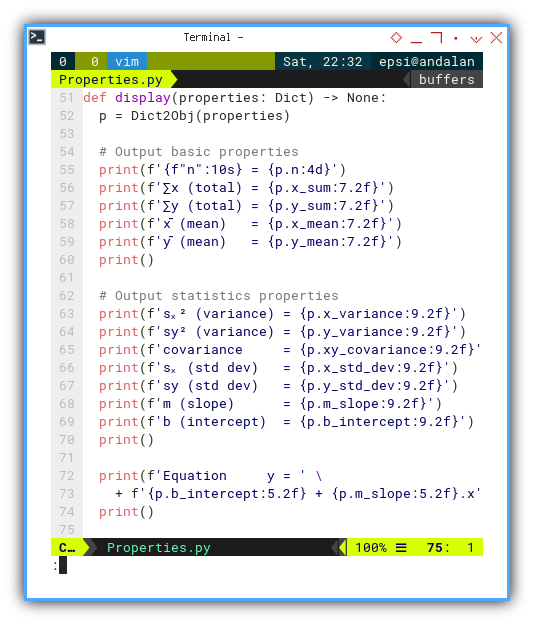
Separation of concerns isn’t just good design. It’s emotional hygiene. Keep our calculations away from our presentation layer.
Using The Helper
In the previous section, we built a reusable statistical Swiss Army knife. Now it’s time to use it, To crunch numbers with elegance and avoid turning our script into spaghetti stats
We’ve tamed the math, now let’s teach it to dance. Let’s go further with other statistical properties.
Python Source
You can find the full script here:
This is where the simple computation meets simple reusability.
Loading The Helper
The get_properties() function bundles everything we need,
from means to regression slopes,
and hands them over in a tidy dictionary.
Then, like a magician pulling rabbits from a hat
(except the rabbits are statistical metrics),
we unpack them into our local workspace.
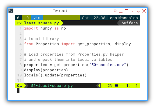
import numpy as np

# Local Library
from Properties import get_properties, display

# Load properties from Properties.py helper
# and unpack them into local variables
properties = get_properties("50-samples.csv")
display(properties)
locals().update(properties)
Maintaining dozens of variables manually is like, keeping track of pigeons in a park. Let Python herd them for us.
Calculate R-squared (R²)
Proceed Further
Now we calculate can proceed other calculation, such as the coefficient of determination.
# Calculate R-squared (R²)
r_squared = r_value ** 2

# Output of correlation calculation

print(f'sₓ (std dev)   = {x_std_dev:9.2f}')
print(f'sy (std dev)   = {y_std_dev:9.2f}')
print(f'r (pearson)    = {r_value:9.2f}')
print(f'R²             = {r_squared:9.2f}')
print()
R² tells us how much of the variation in y,
that we’ve successfully explained with x.
It’s the academic equivalent of a victory lap.
Calculating t-value
Academic Showdown
Once we have residuals,
we can compute the t-value to test the slope’s statistical significance.
It’s like asking, “Hey, β₁, are you real or just random noise?”.
# Create regression line
y_fit = m_slope * x_observed + b_intercept
y_err = y_observed - y_fit

# Calculate variance of residuals (MSE)
var_residuals = np.sum(y_err ** 2) / (n - 2)

# Calculate t-value
t_value = m_slope / std_err_slope

# Output the results
print(f'MSE = ∑ϵ²/(n-2)     = {var_residuals:9.2f}')
print(f'SE(β₁)  = √(MSE/sₓ) = {std_err_slope:9.2f}')
print(f't-value = β̅₁/SE(β₁) = {t_value:9.2f}')
print()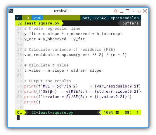
Regression without checking t-values is like,
baking a cake and skipping the taste test.
It might look good, but is it actually meaningful?
Output Result
The final output gives us all the important values at a glance. No need to dive into formulas every time. Our helper did the heavy lifting. How about us? We just sip coffee and interpret.
n          =   13
∑x (total) =   78.00
∑y (total) = 2327.00
x̄ (mean)   =    6.00
ȳ (mean)   =  179.00

sₓ² (variance) =     14.00
sy² (variance) =  23786.00
covariance     =    606.67
sₓ (std dev)   =      3.74
sy (std dev)   =    154.23
m (slope)      =     40.00
b (intercept)  =    -61.00

Equation     y = -61.00 + 40.00.x

sₓ (std dev)   =      3.74
sy (std dev)   =    154.23
r (pearson)    =      0.97
R²             =      0.94

MSE = ∑ϵ²/(n-2)     =   1638.00
SE(β₁)  = √(MSE/sₓ) =      3.00
t-value = β̅₁/SE(β₁) =     13.33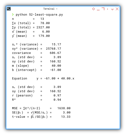
Interactive JupyterLab
Want to poke around and tweak things?
Grab the interactive Jupyter notebook:
A playground where the regression lines are friendly, and the errors politely raise their hands.
Further Library
If you’ve ever wondered how to raise eyebrows, at a party full of statisticians, just whisper:
“I calculated the p-value myself…”
Let’s peek under the hood and manually compute that mysterious number.
Yes, Python makes the calculation of p-value using t_distribution easy,
but understanding the math earns you honorary membership in the
Python Source
Full script available here:
T Distribution
Just forget the helper
First we need to import the t-distribution,
Mote that we do not need Properties helper,
to show how easy it is to obtain the value with python.
import numpy as np
from scipy.stats import linregress
from scipy.stats import t as t_distribution
Now, let’s grab the data:
# Getting Matrix Values
pairCSV = np.genfromtxt("50-samples.csv",
  skip_header=1, delimiter=",", dtype=float)

# Extract x and y values from CSV data
x_observed = pairCSV[:, 0]
y_observed = pairCSV[:, 1]

# Number of data points
n = len(x_observed)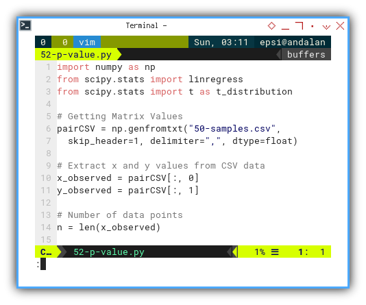
Sometimes it’s refreshing to calculate things manually. Like grinding our own coffee instead of using instant.
Linear Regression
Let’s run a quick regression with linregress,
which kindly gives us the slope, intercept, and standard error,
no questions asked.
# Calculate slope (m), intercept (b),
# and other regression parameters
m_slope, b_intercept, r_value, p_value, \
std_err_slope = linregress(x_observed, y_observed)

# Create regression line
y_fit = m_slope * x_observed + b_intercept
y_err = y_observed - y_fit
This is our first checkpoint.
linregress gives us the t-value and p-value,
but we’ll double-check it ourselves,
just like a paranoid statistician should.
P Value and T Value
Then manually calculate p value using cdf().
# Calculate degrees of freedom
df = n - 2

# Calculate variance of residuals (MSE)
var_residuals = np.sum(y_err ** 2) / (n - 2)

# Calculate t-value
t_value = m_slope / std_err_slope

# Calculate two-tailed p-value
p_value = 2 * (1 - t_distribution.cdf(abs(t_value), df))

# Output the results
print(f'Slope (m): {m_slope:.2f}')
print(f'Standard error of the slope: {std_err_slope:.2f}')
print(f't-value: {t_value:.2f}')
print(f'Two-tailed p-value: {p_value:.10f}')
print()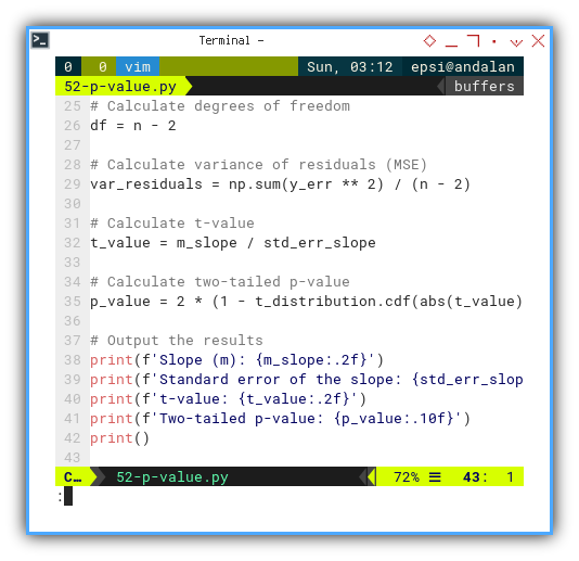
The cdf() function helps us estimate the probability of getting a t-value.
P Value and T Value
The Long Way: trust, but verify. Manual Verification with Critical
t
Let’s pretend we’re suspicious of scipy,
and want to verify everything with our own critical t-table logic.
And also calculate p-value manually using critical t-value,
using ppf and also cdf.
# Define the significance level (alpha)
alpha = 0.05  # for a two-tailed test

# Calculate critical t-value
critical_t = t_distribution.ppf(1 - alpha / 2, df)

# Calculate the p-value manually
td = t_distribution.cdf(abs(t_value), df)
if abs(t_value) > critical_t:
  p_value_manual = 2 * (1 - td)
else:
  p_value_manual = 2 * td

print(f'Critical t-value: {critical_t:.10f}')
print(f'Manually calculated p-value: {p_value_manual:.10f}')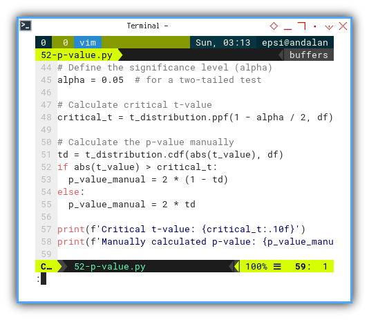
Output Result
And voilà, both automatic and manual methods agree. Our slope is statistically significant, and now we know exactly why.
Slope (m): 40.00
Standard error of the slope: 3.00
t-value: 13.33
Two-tailed p-value: 0.0000000391

Critical t-value: 2.2009851601
Manually calculated p-value: 0.0000000391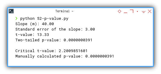
Ask Your Statistician
That’s it for this hands-on walkthrough!
And remember: when in doubt, consult your friendly neighborhood statistician
We’re the only people who get excited over tiny p-values.
Interactive JupyterLab
You can obtain the interactive JupyterLab in this following link:
What’s the Next Exciting Step 🤔?
Now that we’ve crunched the numbers,
danced with t-values, and wrestled with p-values,
it’s time to stop staring at digits,
and see what the data is really trying to say.
Visualization turns abstract math into intuitive insight. It’s the difference between saying, “This line fits pretty well,” and showing a graph that makes your colleagues say, “Ah, now I get it.”
Ready to turn numbers into pictures? Dive into the next chapter: [ Trend - Properties - Visualization ]. Where math meets art, and our regression line finally, gets the spotlight it deserves.