Trend - Least Square

Trend: Prediction

Trend: Regression

Trend: Enhanced

Trend: Language

Local Group

Preface

Goal: Curve fitting examples for daily basis, using least squares method.

I’m not a statistician, though I do occasionally dress like one (corduroy optional). That’s why when I do talk about statistics, I tread carefully.

We will start by laying out the math, because math doesn’t lie, only people misinterpret it. Then move to spreadsheet implementation using Calc (which plays nicely with Excel). And finally round things off with a bit of Python scripting. All practical, all grounded, and no asymptotic nonsense (yet).

From here, we will gracefully tiptoe, into regression analysis and correlation

1: Statistic Notation

Before we hurl ourselves at least squares, we need to brush up on the two pillars of statistical awkwardness: populations (theoretical utopia) vs. samples (your messy spreadsheet data).

Population and Samples

Statistical Properties

Statistic differ between population and samples. For least squares, the calculation is the same, even though the notation is different. For example the Mean notation.

Here’s how statisticians distinguish between perfection and reality:

$\begin{align} \begin{aligned} &\text{Mean (Average):} \\ &\begin{array}{|c|c|} \hline \mathrm{\textbf{Population}} & \mathrm{\textbf{Sample}} \\ \hline \mu = \frac{1}{N}\sum\limits_{i=1}^{N} x_i & \bar{x} = \frac{1}{n}\sum\limits_{i=1}^{n} x_i \\ \hline \end{array} \end{aligned} \end{align}$

Where

μ (mu): The true average, as seen by an all, knowing statistical deity.
x̄ (x-bar): Your best guess, based on whatever you scraped off a CSV file.

Notation impacts formulas, especially when calculating things like variance, regression coefficients, and correlation. Where degrees of freedom lurk, like surprise plot twists in a statistics textbook.

For correlation and regression, the equation has different degree of freedom. This means, the equation is different. We will talk about this later.

2: The Math Behind

Which Least Square

Even least squares come in multiple flavors. Like yogurt, but for math.

When it comes to solving least squares, statisticians have options. And by options, we mean slightly different ways, to arrive at exactly the same answer. Because math, like bureaucracy, loves redundancy.

Here are three friendly paths to the truth:

Direct Equation Derivation: algebra straight from calculus.
Equation Using Means: tidy, intuitive, and easier on the eyes.
Matrix Method: for when you’re feeling fancy (or lazy, thanks to Excel and Python).

Spreadsheet: Workbook with Multiple Worksheet

All three have the same result, and with spreadsheet we can calculate with any method easily. You can choose what equation suitable for your case.

Whichever method you pick, they’ll all walk you to the same solution. That’s the beauty of math. Everyone disagrees on the path, but we all end up at the same sad residuals.

Worksheet Source

Playsheet Artefact

Yes, the spreadsheet exists. And yes, it’s editable. Because what good is math if you can’t poke at it?

github.com/…/math/trend/least-square.xlsx

Go wild. Or at least, copy-paste responsibly.

Slope and Intercept

Let’s say you’ve got a bunch of data points (x, y). You want to find the best straight line that captures their general vibe.

$y = mx + b$

With the same x, from observed value (x,y), we can get the prediction value of y. Now we have two kind of y, the observed value as the calculation source, and the predicted value as the result of the curve fitting equation.

$\begin{array}{|c|c|} \hline x_i & \textbf{observed x} \\ \hline y_i & \textbf{observed y} \\ \hline \hat{y}_i & \textbf{predicted y} \\ \hline \end{array}$

Where:

xᵢ: observed x-values (a.k.a. your independent variable)
yᵢ: observed y-values (the thing you care about)
ŷᵢ: predicted y-values from the fitted line

The fit equation for the predicted y value (ŷᵢ):

$\hat{y}_i = mx_i + b$

Residual

Because data is never fully obedient.

Real-world data never falls perfectly on your line, unless you’re cheating. The residual is the amount by which each point rebels:

The formula for the slope (m) and intercept (b) of the least squares regression line, can be derived from the principle of minimizing the sum of squared errors (residuals) , etween the observed values of y and the values predicted by the regression line.

The residual for each observation is, the difference between the observed value of y and the predicted value of y:

$e_i = y_i - \hat{y}_i$

The sum of squared residuals (SSE) is defined as:

$SSE = \sum\limits_{i=1}^{n} (e_i)^2 = \sum\limits_{i=1}^{n} (y_i - \hat{y}_i)^2$

Our goal is to minimize SSE by choosing appropriate values of m and b To find the values of m and b that minimize SSE, we take the derivatives of SSE with respect to m and b and set them both equal to zero:

$\begin{align*} \frac{\partial SSE}{\partial m} = 0 && \frac{\partial SSE}{\partial b} = 0 \end{align*}$

We take derivatives, and pretend we’re solving for enlightenment.

Direct Equation

Algebra, the Original Regression Tool™

Solving these equations simultaneously will, give us the values of m and b that minimize SSE, hich are the least squares estimates of the slope and intercept.

After some algebraic manipulation, dark magic and friendly spirit, the formulas for m and b can be derived as:

$\begin{align*} m &= \frac{n\sum{xy} - \sum{x}\sum{y}}{n\sum{x^2} - (\sum{x})^2} \\ b &= \frac{\sum{y} - m\sum{x}}{n} \end{align*}$

Great for spreadsheets. Easy to compute. Even easier to impress your manager with.

Equation with Mean

For those who prefer elegance over raw sums.

This version centers around sample means, and offers slightly more interpretable mat (and maybe less typing):

$\begin{align*} m &= \frac{\sum{(x_i - \bar{x})(y_i - \bar{y})}}{\sum{(x_i - \bar{x})^2}} \\ b &= \bar{y} - m\bar{x} \end{align*}$

Perfect if you enjoy statistics and symmetry.

Matrix of System

When your data wants to feel like linear algebra.

Same result, but now it looks smarter. The least squares solution for linear regression can be derived using matrix notation. In matrix notation, the equations are represented as:

$\begin{bmatrix} n & \sum{x_i} \\ \sum{x_i} & \sum{x_i^2} \end{bmatrix} \begin{bmatrix} b \\ m \end{bmatrix} = \begin{bmatrix} \sum{y_i} \\ \sum{x_i y_i} \end{bmatrix}$

Solve m and b using matrix inversion: The solution is given by:

$\begin{bmatrix} b \\ m \end{bmatrix} = \begin{bmatrix} n & \sum{x_i} \\ \sum{x_i} & \sum{x_i^2} \end{bmatrix}^{-1} \begin{bmatrix} \sum{y_i} \\ \sum{x_i y_i} \end{bmatrix}$

Those three are the same least square equations. Those would produce the same result. There are other approach as well in the realm of least square, but let’s skip them this time.

Which Equation Should I Use?

As a summary

Direct formula? Great for worksheets.
Mean-based? More intuitive and elegant.
Matrix form? Flexible, programmable, and scalable.

Use whichever fits your current mood, or spreadsheet layout. Just remember: they all land on the same best-fit line. And that’s the least you can expect from least squares.

3: Direct Solution

Let’s put all that beautiful theory to work, and calculate a real least squares regression line using the direct formula. Time to trade talking for tallying.

Known Values

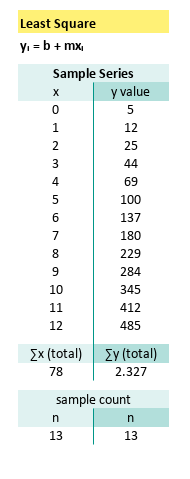
Suppose you’ve collected this pristine (and suspiciously well-behaved) data set:

(x, y) = [(0, 5), (1, 12), (2, 25), (3, 44), (4, 69), (5, 100), (6, 137), (7, 180), (8, 229), (9, 284), (10, 345), (11, 412), (12, 485)]

If that looks like a quadratic curve wearing a linear disguise… Well, you’re not wrong. But remember: we’re only fitting a line, no matter how the data screams otherwise.

First, let’s get our stats straight:

$\begin{align*} n = 13 && \sum x = 78 && \sum y = 2327 && \end{align*}$

For completeness (and spreadsheet nerds), here’s how those quantities are defined:

$\begin{align*} \text{count} = \sum\limits_{i=1}^{n} 1 && \text{sum}_{x} = \sum\limits_{i=1}^{n} x_i && \text{sum}_{y} = \sum\limits_{i=1}^{n} y_i && \end{align*}$

In Excel (or LibreOffice Calc), this translates to plain old =COUNT(...) and =SUM(...). You don’t even need to remember the formulas, just remember where your mouse is.

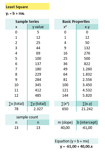
Least Square: Worksheet: Sample Series

Tabular Calculation

Time to bring out the heavy artillery: the direct equation for slope (m) and intercept (b).

$\begin{align*} m &= \frac{n\sum{xy} - \sum{x}\sum{y}}{n\sum{x^2} - (\sum{x})^2} \\ b &= \frac{\sum{y} - m\sum{x}}{n} \end{align*}$

Now, let’s add a few more ingredients to our sum soup. We can calculate further:

$\begin{align*} n &= 13 \\ \sum x &= 78 \\ \sum y &= 2327 \\ \sum (x)^2 &= 650 \\ \sum (x.y) &= 21242 \\ \end{align*}$

Let’s plug it all into the blender (a.k.a. the formula) and see what comes out.

Calculating the Slope (m)

Now we can calculate, the m (slope):

$\begin{align*} m &= \frac{(13 \times 21242) - (78 \times 2327)}{(13 \times 650 - (78)^2} \\ &= \frac{276146 - 181506}{8450 - 6084} \\ &= \frac{94640}{2366} \\ &= 40.0 \end{align*}$

You read that right. Exactly 40. The math gods are smiling.

Calculating the Intercept (b)

And also the b (intercept):

$\begin{align*} b &= \frac{\sum{y} - m\sum{x}}{n} \\ &= \frac{2327 - 40 \times 78}{13} \\ &= \frac{-793}{13} \\ &= -61 \end{align*}$

A negative intercept? Yep. The line starts in debt. Relatable.

Final Regression Equation

Putting it all together, our least-squares linear model is:

$y = -61 + 40x$

This line won’t pass through every point (it’s not supposed to!), but it will minimize the total squared error across all of them. That’s what least squares is all about: fitting best, not perfectly.

Least Square: Worksheet: Direct Equation

With tabular calculation in a spreadsheet, you can arrive at the exact same equation. Now you can see how easy it is, to write down the equation in tabular spreadsheet form.

4: Solution Using Mean

Where averages do all the heavy lifting.

This is easy when you want to combine, with tabular calculation of regression and correlation.

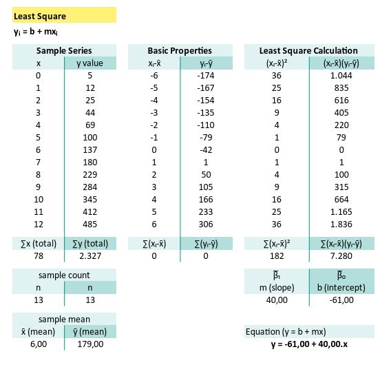
Tabular Calculation

The least squares regression line (y = mx + b), can be found more gracefully using sample means. This method skips some of the clunky summing of products and squares, in favor of centering the data.

Calculate the mean of x and y

$\bar{x} = \frac{1}{n} \sum\limits_{i=1}^{n} x_i$ $\bar{y} = \frac{1}{n} \sum\limits_{i=1}^{n} y_i$

Calculate the slope (m)

$m = \frac{\sum\limits_{i=1}^{n} (x_i - \bar{x})(y_i - \bar{y})}{\sum\limits_{i=1}^{n} (x_i - \bar{x})^2}$

Calculate the y-intercept (b)

$b = \bar{y} - m\bar{x}$

The final equation for the least squares regression line is:

$y = mx + b$

Now let’s calculate the statistic properties for given data point above:

$\begin{align*} n &= 13 \\ \sum x &= 78 \\ \sum y &= 2327 \\ \bar{x} &= 6 \\ \bar{y} &= 179 \\ \end{align*}$

And also:

$\begin{align*} \sum{(x_i - \bar{x})^2} &= 182 \\ \sum{(x_i - \bar{x})(y_i - \bar{y})} &= 7280 \\ \end{align*}$

Now we can calculate, the m (slope):

$\begin{align*} m &= \frac{7280}{182} \\ &= 40.0 \end{align*}$

and the b (intercept):

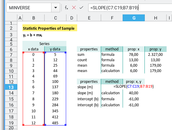
$\begin{align*} b &= \bar{y} - m\bar{x} \\ &= 179 - 40 \times 6 \\ &= -61 \end{align*}$

Spreadsheet View

Tabular calculation in Excel (or Calc) makes this method super approachable, and easier to audit when your regression line goes rogue:

Least Square: Worksheet: Using Means

When your data behaves reasonably (and doesn’t come with drama), this method is clean, elegant, and friendly, even to your future self looking back at the spreadsheet next week.

5: Solution Using Matrix

This is suitable as a basis, when you need to extend to non linier curve fitting.

This method isn’t just for the mathematically elite. It’s the foundation for curve fitting beyond straight lines. Think of it as the gateway drug to polynomial regression, splines, and your favorite buzzword: machine learning.

Tabular Calculation

Matrix form might look intimidating, but under the hood, it’s the same old least squares. It also scales beautifully when you move past linear trends into higher orders.

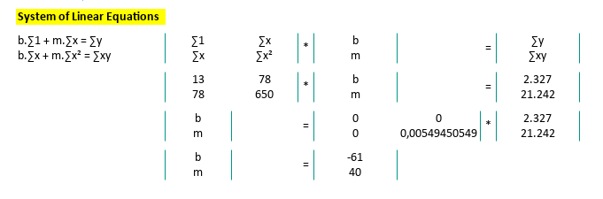
Let’s revisit the matrix equation:

$\begin{bmatrix} n & \sum{x_i} \\ \sum{x_i} & \sum{x_i^2} \end{bmatrix} \begin{bmatrix} b \\ m \end{bmatrix} = \begin{bmatrix} \sum{y_i} \\ \sum{x_i y_i} \end{bmatrix}$

Yes, this is still the good old y = mx + b, just dressed up in its linear algebra tuxedo.

Now, applying actual numbers from our trusty dataset, getting the m (slope) and b(intercept), using matrix inversion.

$\begin{array}{cc} & \begin{bmatrix} 13 & 78 \\ 78 & 650 \end{bmatrix} \begin{bmatrix} b \\ m \end{bmatrix} = \begin{bmatrix} 2327 \\ 21242 \end{bmatrix} \\ \Rightarrow & \begin{bmatrix} b \\ m \end{bmatrix} = \begin{bmatrix} 13 & 78 \\ 78 & 650 \end{bmatrix}^{-1} \begin{bmatrix} 2327 \\ 21242 \end{bmatrix} = \begin{bmatrix} -61 \\ 40 \end{bmatrix} \end{array}$

We arrive at the same solution as before:

Slope (m) = 40, Intercept (b) = -61

Linear algebra: different route, same destination. Except this road is paved for scaling up.

Spreadsheet View

Even Excel’s formula engine can handle this with a few matrix tricks: MMULT, MINVERSE, and the occasional coffee break while debugging array formulas.

Least Square: Worksheet: Using Matrix

Why It’s a Big Deal

While you might not need the matrix form for a single line, it’s your golden ticket when the model evolves:

Need to fit a parabola? Matrix.
Multiple x variables? Matrix.
Polynomial regression with terms up to x^10? You guessed it. Matrix.

Neo had to choose the red pill. You? You just need MINVERSE().

6: Built-in Formula

When you love stats, but also love letting Excel do the heavy lifting.

Let’s be honest: sometimes we don’t want to manually crank, through all the sums, products, and parentheses. Sometimes, we want to tell our spreadsheet, “Figure it out,” and let the magic happen.

The good news is, Excel (or Calc, if you’re open source and proud) has use covered.

First Things First

The Basics

Before jumping to the fancy built-ins, let’s warm up with the classics.

Least Square: Worksheet: Using Matrix

Grab the totals and averages for x and y, like you’re stretching before a marathon of regression.

Properties	x Formula	y Formula
Total	=SUM(B7:B19)	=SUM(C7:C19)
Count	=COUNT(B7:B19)	=COUNT(C7:C19)
Mean	=AVERAGE(B7:B19)	=AVERAGE(C7:C19)

Even if we’re using AVERAGE, it’s good practice to know the underlying logic. Especially if we’ll be coding this later, in Python, R, or whispering to pandas.

In fact, here’s how we can calculate the mean without AVERAGE (yes, sometimes we like to flex on basic functions):

Properties	Formula
Mean x	=SUM(B7:B19)/COUNT(B7:B19)
Mean y	=SUM(C7:C19)/COUNT(C7:C19)

Built-in Regression

No Pain, All Gain

Now we get to the really lazy part. I mean efficient, part. Excel has built-in regression functions, that give use slope and intercept in one clean shot.

Just remember: for array operation formulas, hit Ctrl+Shift+Enter or Excel will pretend you never asked.

Properties	Formula
slope (m)	{=SLOPE(C7:C19;B7:B19)}
intercept (b)	{=INTERCEPT(C7:C19;B7:B19)}

If we’re testing many data sets or building a dashboard, these functions are fast, reliable, and save us from spreadsheet-induced carpal tunnel.

For the Brave

Manual Calculation

Want to see how the built-ins work under the hood? Try calculating it yourself using mean-centered values:

Properties	Formula
slope (m)	=SUM((B7:B19 - G10)*(C7:C19 - H10))/SUM((B7:B19 - G10)^2)
intercept (b)	=H9-G14*G9

We’re subtracting the mean, multiplying, summing, conducting a tiny symphony of statistics.

Final Thoughts

That’s it for now. Whether we’re letting Excel take the wheel, or crunching numbers the old-fashioned way, we’ve got solid tools for fitting a line.

Next up? We will turn the volume up, and explore regression and correlation. Dive into more complex formula, where the real drama of data begins.

7: Python

So, what’s happened when, spreadsheets just aren’t satisfying, for our craving for automation and repeatability.

Python offers several ways to perform least squares regression, ranging from the “I trust NumPy with my life” approach, to “let’s see the residuals and p-values too, please.”

We’ll look at:

numpy.polyfit or Polynomial.fit: Quick and clean.
scipy.stats.linregress Lightweight but statistically aware.
statsmodels.api.OLS Heavy artillery for full statistical modeling.

You can follow along with the full script here:

github.com/…/trend/41-least-square.py

Let’s start with some data. Think of this as our patient zero in a curve-fitting, during current pandemic.

# Given data
x_values = np.array(
  [0, 1, 2, 3, 4, 5, 6, 7, 8, 9, 10, 11, 12])
y_values = np.array(
  [5, 12, 25, 44, 69, 100, 137,
    180, 229, 284, 345, 412, 485])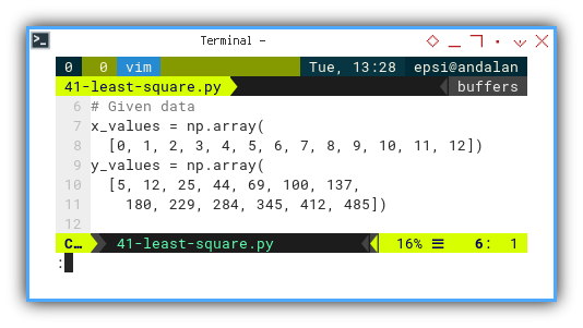

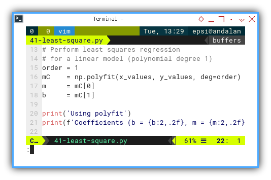
Python: Built-In: Curve Fitting: Data Series

Polyfit

Fast, friendly, and polynomial-curious.

If you just want the best-fit line, and don’t need to explain it to your thesis advisor, numpy.polyfit is your go-to.

import numpy as np

# Perform least squares regression
# for a linear model (polynomial degree 1)
order = 1
mC    = np.polyfit(x_values, y_values, deg=order)
m     = mC[0]
b     = mC[1]

print('Using polyfit')
print(f'Coefficients (b = {b:2,.2f}, m = {m:2,.2f})\n')

Quick prototyping. Great for trendlines. And yes, it works for higher-degree polynomials too. Just in case our data starts curving like a rollercoaster.

Python: Built-In: Curve Fitting: Polyfit

Note: Please be prepate for polyfit replacement called Polynomial.fit.

Linregress

Like polyfit, but wears a lab coat.

scipy.stats.linregress gives us slope, intercept, and bonus goodies like r-value and standard error. Use it when we want our math to sound more “peer-reviewable.”

from scipy import stats

# SciPy: scientific computing built on top of NumPy.
m, b, _, _, _ = stats.linregress(x_values, y_values)

print('Using linregress')
print(f'Coefficients (b = {b:2,.2f}, m = {m:2,.2f})\n')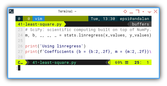

Python: Built-In: Least Square: Linear Regression

Ideal for statistical analysis with minimal fuss. Also lets us pretend we’re doing something much more complicated than we are.

OLS

Sometimes we want the full regression buffet, not just the drive-thru.

For those of us who like residual plots, confidence intervals, and enough statistical output to paper a conference, statsmodels has us covered.

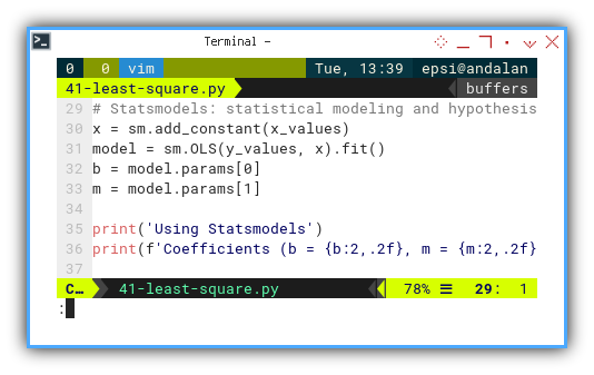
import statsmodels.api as sm

# Statsmodels: statistical modeling and hypothesis testing.
x = sm.add_constant(x_values)
model = sm.OLS(y_values, x).fit()
b = model.params[0]
m = model.params[1]

print('Using Statsmodels')
print(f'Coefficients (b = {b:2,.2f}, m = {m:2,.2f})\n')

This is the professional toolkit. We will want this when we start checking assumptions, diagnosing models, or trying to impress our statistical consultant.

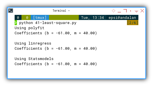
Python: Built-In: Least Square: Stats Models: OLS

And voilà, no matter how we slice it. NumPy, SciPy, or Statsmodels, we end up with the same tidy equation:

Using polyfit
Coefficients (b = -61.00, m = 40.00)

Using linregress
Coefficients (b = -61.00, m = 40.00)

Using Statsmodels
Coefficients (b = -61.00, m = 40.00)

Consistent results across different tools is a great sanity check, especially if our sanity depends on reproducible results.

Python: Built-In: Least Square: Output Result

There is no need for fancy chart plot this time.

You can obtain the interactive JupyterLab in this following link:

github.com/…/trend/41-least-square.ipynb

Manual Calculation

For the Purists

When deep down, you don’t trust functions, unless you’ve re-derived them in a dimly lit lab.

Let’s go back to first principles. Here’s how we’d do it ourself. No black boxes, just beautiful algebra.

github.com/…/trend/42-least-square.py

First we calculate basic statistic properties.

# Number of data points
n = len(x_values)

# Calculate sums
sum_x = np.sum(x_values)
sum_y = np.sum(y_values)

# Calculate means
mean_x = np.mean(x_values)
mean_y = np.mean(y_values)

# Output of basic properties
print(f'n = {n:5d}')
print(f'∑x (total) = {sum_x:7.2f}')
print(f'∑y (total) = {sum_y:7.2f}')
print(f'x̄ (mean)   = {mean_x:7.2f}')
print(f'ȳ (mean)   = {mean_y:7.2f}')
print()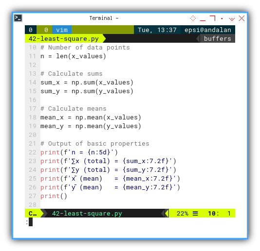

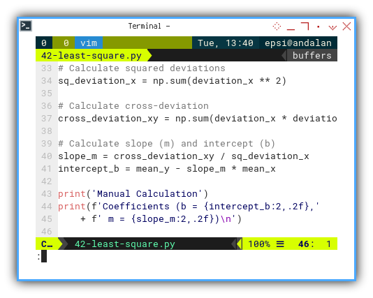
Python: Manual Calculation: Least Square: Mean Properties

Then go further, bring in the deviations:

# Calculate deviations
deviation_x = x_values - mean_x
deviation_y = y_values - mean_y

# Calculate squared deviations
sq_deviation_x = np.sum(deviation_x ** 2)

# Calculate cross-deviation
cross_deviation_xy = np.sum(deviation_x * deviation_y)

# Calculate slope (m) and intercept (b)
slope_m = cross_deviation_xy / sq_deviation_x
intercept_b = mean_y - slope_m * mean_x

print('Manual Calculation')
print(f'Coefficients (b = {intercept_b:2,.2f},'
    + f' m = {slope_m:2,.2f})\n')

Manual calculation reinforces understanding of the math behind the tools. Also, great for debugging or impressing our coworkers with a “I did this without NumPy” moment.

Python: Manual Calculation: Least Square: Deviation Properties

And here’s the proof it worked:

n =    13
∑x (total) =   78.00
∑y (total) = 2327.00
x̄ (mean)   =    6.00
ȳ (mean)   =  179.00

Manual Calculation
Coefficients (b = -61.00, m = 40.00)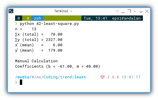

Python: Manual Calculation: Least Square: Result Output

Need to test or tinker interactively? Fire up these Jupyter Notebooks and experiment like a modern-day Gauss:

github.com/…/trend/42-least-square.ipynb

We take this straight line obsession further, with regression, correlation, and maybe even the mysterious world of non-linear fitting. Are you ready to curve things up?

Where Do We Go From Here 🤔?

Now that we’ve bravely tamed the Least Squares beast, let’s talk about what lies ahead in our adventure.

We’ve taken a mathematical equation, made it practical (because who doesn’t love practical?), turned it into a neat spreadsheet (tabular bliss, am I right?), and even whipped up some Python code. That’s like the statistical equivalent of baking a cake from scratch, but with fewer crumbs and more data insights.

And the best part? It’s fun, right? The kind of fun that only comes from numbers and formulas working together, like a well-oiled machine. Ah, the joy of regression lines…

Now that we’ve conquered the basics, we can explore even more statistical properties. Regression and correlation are just the beginning. We can dig deeper into the data, and start exploring how variables relate to each other, why they relate (or don’t), and how much faith we can place in our model’s predictions. Trust but verify, that’s the statistician’s mantra.

But don’t worry, the journey isn’t over yet! If we’re still hungry for more statistical wizardry, take a detour over to [ Trend - Properties - Cheatsheet ].

It’s like the ultimate guidebook for your next steps in the land of data trends.