Preface
Goal: Implement polynomial equation in worksheet. From theory to data modelling in Excel/Calc. Solving third order polynomial equation.
Welcome to the world where algebra meets the almighty spreadsheet.
Here, we take our polynomial equations out of their theoretical ivory tower, and drop them right into Excel or LibreOffice Calc, where real-world data lives (and occasionally misbehaves).
This isn’t abstract math for fun. Okay, also for fun, but it’s primarily about learning, how to actually do polynomial regression, in the software many people already use every day.
We’ll walk through the special case of cubic equations. Why cubic? Because it’s the perfect mix of complexity and practicality. Also, it sounds cooler than quadratic.
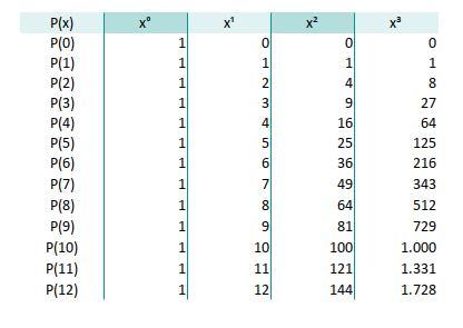
Tabular layout helps build intuition:
you see the powers of x, the sums, the coefficients.
It’s like watching a matrix do interpretive dance,
surprisingly insightful.
Shorter
But Wait… There’s a Shortcut!
Spreadsheets have a magical formula called LINEST,
which can solve everything in one go.
But we’re not using it.
Why? Because the goal here is understanding,
not just button-mashing.
Plus, LINEST feels like cheating…
and we’re classy statisticians.
Instead, we will derive the solution by hand (well, by Excel and Python). We are going to calculate the solution manually. The step by step approach is required to get deeper understanding, of how things works. So the next time someone casually mentions “least squares regression” we will nod confidently, and not just hope they change the subject.
Shifting from Interpolation
From Interpolation to Approximation
Here’s the twist, in previous articles, we connected exact points with a polynomial (interpolation). Now, we’re entering the realm of curve fitting. Modeling data that doesn’t play nice.
The math shifts slightly, because we now have more data points than coefficients. So, we need a clever workaround to make our matrix solvable.
Enter the transpose trick
The difference with previous interpolation is,
the approach of getting the matrix solution.
Since inverse can only work with square nxn matrix.
We need to alter the equation a bit with transpose.
This technique (also known as the normal equation) is, the foundation of least squares regression, which is the backbone of many machine learning models, economic forecasts, and awkwardly plotted trendlines in presentations.
Manual Labor
But Make It Fun
We’re skipping the spreadsheet autopilot and doing things manually. Because reverse-engineering builds true understanding.
Here’s a preview of the spreadsheet we’ll build:
Later, we’ll recreate the same logic in Python,
not because we dislike polyfit,
but because we like knowing what it`s doing behind the scenes.
After all, any statistician can click a button, but a real statistician knows why that button works.
Step by Step
We’ll focus on a third-order polynomial (a + bx + cx² + x³) and walk through each step methodically:
We would pick third order polynomial as a case. Then we would explain in systematic way.
-
Start with cubic equation with know coefficient, to produce Y-value, using spreadsheet.
-
Solve the Y-Value, using spreadsheet, but this time with the help of matrix (reverse-engineer the coefficients).
-
Inverse using spreadsheet, find the coefficient, with know Y-Value. (Yes, Excel can do it. No, it’s not sorcery)
-
Translate the entire matrix process into Python code.
We will leave this with more than just answers. We will understand the process, which is exactly what separates a spreadsheet user from a spreadsheet wizard.
Worksheet Source
A little Excel playground for the mathematically curious.
You can grab the Excel file, explore, and even break things. It’s encouraged, in a safe, learning sort of way.
1: Polynomial Case
Task: Find the coefficient.
This is where math meets detective work. We’re using numerical methods to solve a statistical puzzle: Find the coefficients of a cubic polynomial, that best explains a set of known values.
Polynomial Expression
Let’s start with the usual suspect: a third-degree (cubic) polynomial.
Here, a, b, c and d are the coefficients we’re after.
You could say they’re the polynomial’s DNA.
If we know them, we know everything.
Known Data
In the real world, you rarely get handed perfect equations. Instead, you’re given data, and expected to find the pattern. Our mission is to find the coeffient, based on known data.
For example, here’s our mystery dataset, 13 pairs of (x, y) values:
| X | Y-Value |
|---|---|
| 0 | 5 |
| 1 | 10 |
| 2 | 410 |
| 3 | 90 |
| 4 | 190 |
| 5 | 350 |
| 6 | 460 |
| 7 | 960 |
| 8 | 1050 |
| 9 | 1740 |
| 10 | 1340 |
| 11 | 3270 |
| 12 | 3540 |
This is the kind of messiness you get in actual data science or forecasting work. The goal is to find a polynomial model that fits the trend, even if it doesn’t hit every point.
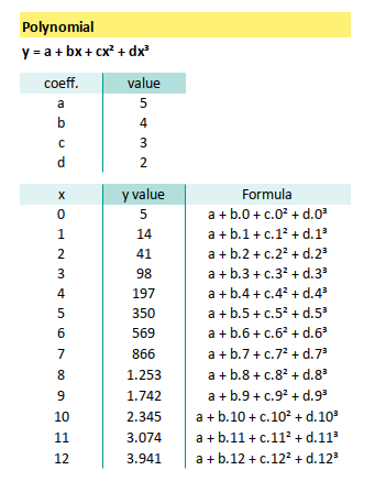
2: Cubic Equation
Let’s warm up by flipping the problem around: What if we already know the coefficients?
| Coeff. | Value |
|---|---|
| a | 5 |
| b | 4 |
| c | 3 |
| d | 2 |
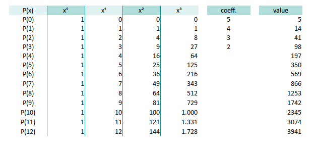
Consider reverse our task, find the data for known coefficient.
Equation
Plug those in and you get the equation:
For the LaTeX crowd, here’s your moment of glory:
y = 5 + 4{x} + 3{x}^2 + 2{x}^3Applying Equation
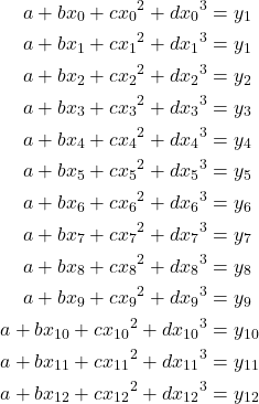
Applying equation for each pairs can be written as below:
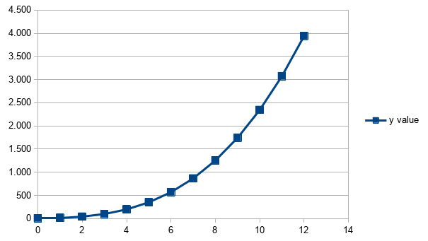
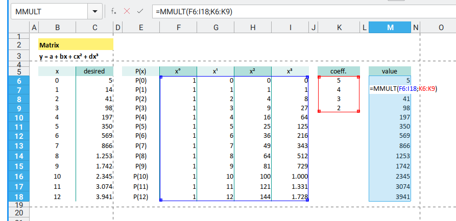
Spreadsheet
Here’s how we bring this math into Excel/Calc.
In the same sheet, we can also visualize the XY line, in a tidy chart as below figure:
We’ve built the equation forward, from coefficients to values. Next, we’ll crank things in reverse and solve, from values to coefficients, using matrix methods.
Stay tuned, we’re about to make Excel do linear algebra, and live to tell the tale.
3: Matrix Equation
Getting unknown Y-Value
Our objective is to reverse-engineer the coefficients. Like CSI: Polynomial Edition.
Now that we’ve seen how a polynomial generates values, let’s flip the problem: We know the outputs (the Y-values), and we want to deduce the equation that made them.
Time to bring in matrices, the Swiss Army knife of numerical methods.
Spreadsheet Setup
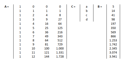
Let’s roll out the big guns:
a 13×4 matrix to represent our polynomial basis.
Multiply this with a 4×1 column matrix of coefficients [a, b, c, d],
and voilà — you get a 13×1 column matrix of Y-values.
Where:
- A is our Vandermonde matrix
- C is our coefficient mystery box
- B is our known Y-values
In Excel, use the MMULT function for matrix multiplication.
Just remember: this isn’t your typical lazy formula,
it needs array calculation.
Use Ctrl+Shift+Enter to activate array mode.
for example for this {=MMULT(F6:I18;K6:K9)} formula.
Now we are ready to solve our real problem.
Reverse back to unknown coefficient for known Y-Value.
This process forms the backbone of many modern statistical and machine learning algorithms. From linear regression to curve fitting. Understanding this helps you move beyond “click-and-hope” analytics.
Our Equation
Vandermonde Matrix
Tthe Vandermonde Matrix sounds fancy, but it’s just powers of X arranged in rows.
Here’s the mathematical form of our 13×4 matrix setup:
The 13x4 size matrix can be described as:
- 13 number of data.
- 4 coefficient, for third order.
For our fellow LaTeX nerds (no judgment, only respect),
you can get the equation by right click the equation above,
and copy the TeX Commands to clipboard from the menu.
This layout, a Vandermonde matrix, is the foundation for polynomial regression and interpolation. It’s how machines (and humans with Excel) learn trends from raw numbers.
4: Inverse Matrix
Getting unknown coefficient
We’ve assembled our matrix. We’ve multiplied it, transposed it, maybe even stared at it until it blinked first. Now, it’s time for the final boss of matrix operations: inversion.
Let’s find those coefficients, the statistical Rosetta Stones that connect Xₛ to Yₛ.
Problem Domain
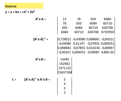
Here’s how our equation looks in the land of spreadsheets:
You might think this looks intense. But to a statistician, this is just Tuesday.
Equation
Let’s start with the basic setup. We are going to solve the formula above using this equation
Now here’s the catch: you can’t invert a non-square matrix. Trying to do that is like asking your toaster to make ice cubes, mathematically forbidden.
Inverse can only work with square nxn matrix.
Since our 13x4 matrix is definitely not a square matrix.
We need to alter the equation a bit with transpose.
This technique is called the Normal Equation. It’s used in linear regression, machine learning, and even AI training. It’s the statistical equivalent of a Swiss watch mechanism. Elegant, precise, and quietly powerful.
LaTeX
If you are curious, the LaTeX code can be obtained by right click the equation. A menu will be shown-up, then you can copy to clipboard.
Want to copy that juicy equation into your own LaTeX editor? Here you go:
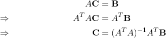
\begin{align*}
              &&    A\mathbf{C}     &= \mathbf{B} \\
  \Rightarrow &&    A^T A\mathbf{C} &= A^T \mathbf{B} \\
  \Rightarrow &&    \mathbf{C}      &= (A^T A)^{-1} A^T \mathbf{B}
\end{align*}
Or use the friendly folks at quicklatex for instant render magic.
Transpose
With transpose formula such as: =TRANSPOSE(E9:H21),
we can have the matrix transposed as below:
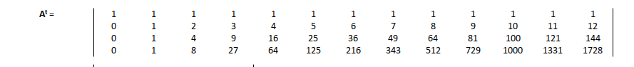
Suddenly, rows become columns. It’s matrix yoga.
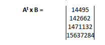
Multiply Like a Pro
Again, we can cross multiply both, with MMULT.
You’ve done this before. MMULT is back. First, let’s do:
- Aᵀ × A
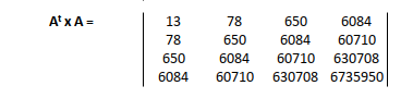
- Aᵀ × B
Statisticians call this the setup for the Normal Equation. Normal in name, but not in workload.
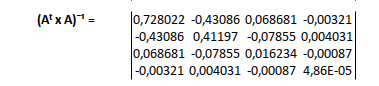
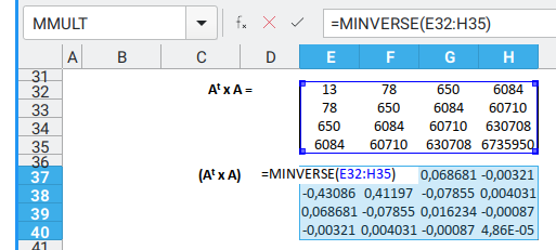
Inverse
To invert the matrix,
we unleash Excel’s MINVERSE formula,
such as {=MINVERSE(E32:H35)}.
Curly brackets mean it’s an array formula. Yes, the ones that need Ctrl+Shift+Enter.
You can examine the excel formula here.
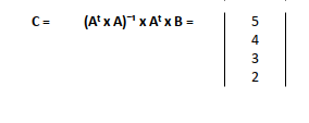
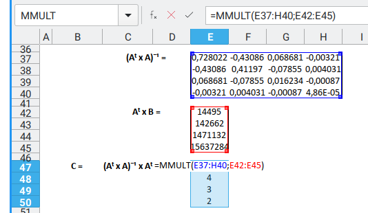
Coeffecient
Multiply the inverse matrix with Aᵀ × B using MMULT, and behold.
The hidden polynomial coefficients rise from the spreadsheet.
You can examine the excel formula here.
Yes, we have our result. It’s official. Our spreadsheet just did algebra.
Big Picture
Here’s how it all connects, spreadsheet-style:
![Polynomial: Excel Matrix: Big Picture][152-polycats-03]
This matrix inversion trick, especially when used with AᵀA, is the backbone of least squares regression, the statistical bread-and-butter of modern data analysis. Whether you’re building a machine learning model, or fitting a curve to cat weight vs. lasagna intake, this method is everywhere.
What’s Our Next Endeavor 🤔?
We’ve done it, We’ve summoned the power of matrix algebra inside a spreadsheet. That alone earns use nerd points redeemable in most academic circles.
But what if our data grows… and our spreadsheet crashes? 😱
That’s where Python enters the scene, cape fluttering, NumPy blazing.
Let’s take those same polynomial calculations, and power them with less-clicking tools called Python, more scaling, and bonus: prettier plots.
Continue here: [ Trend - Polynomial in Python ].