Trend - Polynomial Algebra

Preface

Goal: Understanding how the polynmial internally works. Gently explanation from each form to generalization.

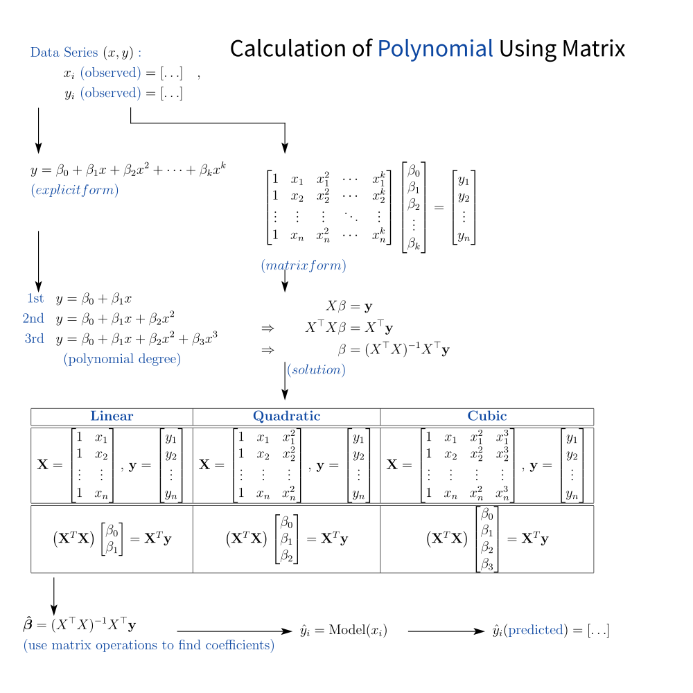
To ease you into the world of equations, here’s a visual roadmap of where we’re heading that outlines the flow of polynomial calculations:

Don’t worry about the equations. Ignore the symbols for now, unless you’re fluent in Matrices. I will start gently, step by step. We’ll walk through it all. No calculus-induced trauma required.

Don’t panic. This is math, not a mystery novel.

---

1: Equation Breakdown

So, you’re still here? Excellent.

That means you’re either really into math, or you’re procrastinating on something else.

Now for the curious. Let’s peel back the curtain and look at the structure behind polynomial regression. Think of this as opening the hood of your regression model. Sure, it runs, but don’t you want to know why it runs?

We’ll eventually tie this into how Excel and Python handle polynomial fitting. For now, let’s admire some good old-fashioned matrix wizardry.

Let’s have a look again to this equation. We are going to connect polynomial equation to regression equation later.

$$\begin{aligned} && A \cdot \mathbf{C} &= \mathbf{B} \\ \Rightarrow && A^\top \cdot A \cdot \mathbf{C} &= A^\top \cdot \mathbf{B} \\ \Rightarrow && \mathbf{C} &= (A^\top A)^{-1} \cdot (A^\top \mathbf{B}) \end{aligned}$$

This is the canonical form of least squares regression. Then what is this (Aᵗ x A) x C = Aᵗ x B looks like in the matrix? We are going to show the gram matrix (Aᵗ.A) of the system.

This equation helps us find the regression coefficients, that minimize the sum of squared errors. The holy grail of fitting.

Linear Regression

Let’s start with the first polynomial boss: the line.

1. Generic Matrix

$$A = \begin{bmatrix} 1 & x_1 \\ 1 & x_2 \\ 1 & x_3 \\ \vdots & \vdots \\ 1 & x_n \\ \end{bmatrix}$$

This matrix A is what we call a design matrix. Yes, statisticians get to “design” things too. Mostly equations and sleep schedules.

2. Normal Equation

$$\begin{aligned} (\mathbf{A}^T \cdot \mathbf{A}) \cdot \begin{bmatrix} a \\ b \\ \end{bmatrix} = \mathbf{A}^T \cdot \mathbf{B} \end{aligned}$$

3. Expanded

   • This equation relate to least square.
   • Now you have alternative way to simplify the matrix calculation in Excel.

$$\begin{bmatrix} n & \sum x_i \\ \sum x_i & \sum x_i^2 \end{bmatrix} \begin{bmatrix} a \\ b \end{bmatrix} = \begin{bmatrix} \sum y_i \\ \sum x_i y_i \end{bmatrix}$$

This gives us a system of two equations in two unknowns. Very solvable. Very spreadsheet-friendly.

4. Inverse (Aᵗ.A)ˉ¹

   • We can cheat the computation for the inverse using this formula.

$$(A^T A)^{-1} = \frac{1}{n \sum x_i^2 - (\sum x_i)^2} \begin{bmatrix} \sum x_i^2 & -\sum x_i \\ -\sum x_i & n \end{bmatrix}$$

No regression article is complete without the classic “look, Ma, I inverted a matrix” moment. Butctually, the inverse equation is not really useful to simplify current tabular calculation, except for curiosity purpose. I’d rather use current excel formula or python.

While you can compute this by hand, I recommend doing it only when your Excel crashes, and you need to impress a statistician at a party.

Quadratic Regression

Welcome to degree two. This is where our nice straight line puts on a little flair.

1. Generic Matrix

$$A = \begin{bmatrix} 1 & x_1 & x_1^2 \\ 1 & x_2 & x_2^2 \\ 1 & x_3 & x_3^2 \\ \vdots & \vdots & \vdots \\ 1 & x_n & x_n^2 \\ \end{bmatrix}$$

2. Normal Equation

$$\begin{aligned} (\mathbf{A}^T \cdot \mathbf{A}) \cdot \begin{bmatrix} a \\ b \\ c \\ \end{bmatrix} = \mathbf{A}^T \cdot \mathbf{B} \end{aligned}$$

3. Expanded

   • Now you have alternative way to simplify the matrix calculation in Excel.

$$\begin{bmatrix} n & \sum x_i & \sum x_i^2 \\ \sum x_i & \sum x_i^2 & \sum x_i^3 \\ \sum x_i^2 & \sum x_i^3 & \sum x_i^4 \end{bmatrix} \begin{bmatrix} a \\ b \\ c \end{bmatrix} = \begin{bmatrix} \sum y_i \\ \sum x_i y_i \\ \sum x_i^2 y_i \end{bmatrix}$$

4. Inverse

   • No easy cheat, we need to compute.

$$(A^T A)^{-1} = \begin{bmatrix} * & * & * \\ * & * & * \\ * & * & * \end{bmatrix}$$

No closed-form shortcut here. Time to break out NumPy or let Excel’s LINEST handle it. Or pray. Both work.

Cubic Regression

Polynomials of degree three: when your line just has to loop.

1. Generic Matrix

$$A = \begin{bmatrix} 1 & x_1 & x_1^2 & x_1^3 \\ 1 & x_2 & x_2^2 & x_2^3 \\ 1 & x_3 & x_3^2 & x_3^3 \\ \vdots & \vdots & \vdots & \vdots \\ 1 & x_n & x_n^2 & x_n^3 \\ \end{bmatrix}$$

2. Normal Equation

$$\begin{aligned} (\mathbf{A}^T \cdot \mathbf{A}) \cdot \begin{bmatrix} a \\ b \\ c \\ d \\ \end{bmatrix} = \mathbf{A}^T \cdot \mathbf{B} \end{aligned}$$

3. Expanded

   • Now you have alternative way to simplify the matrix calculation in Excel.

$$\begin{bmatrix} n & \sum x_i & \sum x_i^2 & \sum x_i^3 \\ \sum x_i & \sum x_i^2 & \sum x_i^3 & \sum x_i^4 \\ \sum x_i^2 & \sum x_i^3 & \sum x_i^4 & \sum x_i^5 \\ \sum x_i^3 & \sum x_i^4 & \sum x_i^5 & \sum x_i^6 \end{bmatrix} \begin{bmatrix} a \\ b \\ c \\ d \end{bmatrix} = \begin{bmatrix} \sum y_i \\ \sum x_i y_i \\ \sum x_i^2 y_i \\ \sum x_i^3 y_i \end{bmatrix}$$

4. Inverse

   • No easy cheat, we need to compute.

$$(A^T A)^{-1} = \begin{bmatrix} * & * & * & * \\ * & * & * & * \\ * & * & * & * \\ * & * & * & * \end{bmatrix}$$

At this point, we’re better off trusting the robots. Let Python do the math, and we focus on making the plots look pretty.

Cheatsheet

Vandermonde

If you remember one thing, remember this: polynomial regression is just linear regression in disguise, wearing powers of x like a fashionable scarf.

Finally summarized in just one table.

$$\begin{equation*} \scriptsize \begin{array}{|c|c|c|} \hline \textbf{Linear} & \textbf{Quadratic} & \textbf{Cubic} \\ \hline \hline \mathbf{A} = \begin{bmatrix} 1 & x_1 \\ 1 & x_2 \\ \vdots & \vdots \\ 1 & x_n \\ \end{bmatrix}, \, \mathbf{B} = \begin{bmatrix} y_1 \\ y_2 \\ \vdots \\ y_n \\ \end{bmatrix} & \mathbf{A} = \begin{bmatrix} 1 & x_1 & x_1^2 \\ 1 & x_2 & x_2^2 \\ \vdots & \vdots & \vdots \\ 1 & x_n & x_n^2 \\ \end{bmatrix}, \, \mathbf{B} = \begin{bmatrix} y_1 \\ y_2 \\ \vdots \\ y_n \\ \end{bmatrix} & \mathbf{A} = \begin{bmatrix} 1 & x_1 & x_1^2 & x_1^3 \\ 1 & x_2 & x_2^2 & x_2^3 \\ \vdots & \vdots & \vdots & \vdots \\ 1 & x_n & x_n^2 & x_n^3 \\ \end{bmatrix}, \, \mathbf{B} = \begin{bmatrix} y_1 \\ y_2 \\ \vdots \\ y_n \\ \end{bmatrix} \\ \hline \hline \left(\mathbf{A}^T \mathbf{A}\right) \begin{bmatrix} a \\ b \\ \end{bmatrix} = \mathbf{A}^T \mathbf{B} & \left(\mathbf{A}^T \mathbf{A}\right) \begin{bmatrix} a \\ b \\ c \\ \end{bmatrix} = \mathbf{A}^T \mathbf{B} & \left(\mathbf{A}^T \mathbf{A}\right) \begin{bmatrix} a \\ b \\ c \\ d \\ \end{bmatrix} = \mathbf{A}^T \mathbf{B} \\ \hline \hline \begin{bmatrix} n & \sum x_i \\ \sum x_i & \sum x_i^2 \\ \end{bmatrix} \begin{bmatrix} a \\ b \\ \end{bmatrix} = \begin{bmatrix} \sum y_i \\ \sum x_i y_i \\ \end{bmatrix} & \begin{bmatrix} n & \sum x_i & \sum x_i^2 \\ \sum x_i & \sum x_i^2 & \sum x_i^3 \\ \sum x_i^2 & \sum x_i^3 & \sum x_i^4 \\ \end{bmatrix} \begin{bmatrix} a \\ b \\ c \\ \end{bmatrix} = \begin{bmatrix} \sum y_i \\ \sum x_i y_i \\ \sum x_i^2 y_i \\ \end{bmatrix} & \begin{bmatrix} n & \sum x_i & \sum x_i^2 & \sum x_i^3 \\ \sum x_i & \sum x_i^2 & \sum x_i^3 & \sum x_i^4 \\ \sum x_i^2 & \sum x_i^3 & \sum x_i^4 & \sum x_i^5 \\ \sum x_i^3 & \sum x_i^4 & \sum x_i^5 & \sum x_i^6 \\ \end{bmatrix} \begin{bmatrix} a \\ b \\ c \\ d \\ \end{bmatrix} = \begin{bmatrix} \sum y_i \\ \sum x_i y_i \\ \sum x_i^2 y_i \\ \sum x_i^3 y_i \\ \end{bmatrix} \\ \hline \end{array} \end{equation*}$$

Check out the handy table above for quick reference. If this looks intimidating, just remember, It’s all just a bunch of sums and products. Like grocery shopping, but with less walking.

Excel, Python, R, they all use versions of this math under the hood. Understanding it helps us trust the output… and debug when things go sideways.

You can see the detail in Wiki with topic of Vandermonde and Least Square.

$$\boxed{ \begin{array}{c} \text{Vandermonde-based least squares} \\ \scriptstyle\text{(Ref: Wikipedia, 2020)} \end{array} }$$

That’s all how the expanded matrix looks like.

---

2: Generalization

Form practical examples, we goes back to conceptual. using standard statistical notation, to avoid confusion.

Statistical Notation

We’ve wandered through the world of polynomial fitting. Linear, quadratic, cubic, and now it’s time to climb the final hill: generalization. Don’t worry, this is the part where everything gets suspiciously neat and the math starts wearing a tuxedo.

Let’s dress up our formulas using standard statistical notation. Why? Because eventually someone will ask you about “β coefficients” at a conference, and you don’t want to just smile and nod.

Explicit Form

This is the classic polynomial regression model. Fancy, formal, and ready for publication.

$$y = \beta_0 + \beta_1 x + \beta_2 x^2 + \cdots + \beta_k x^k$$

This is the function we’re trying to fit. It’s your best guess of how x and y are dancing together. Now with choreography up to degree k.

Matrix Form

Ah, matrices. The universal language of statisticians and robots.

$$\begin{bmatrix} 1 & x_1 & x_1^2 & \cdots & x_1^k \\ 1 & x_2 & x_2^2 & \cdots & x_2^k \\ \vdots & \vdots & \vdots & \ddots & \vdots \\ 1 & x_n & x_n^2 & \cdots & x_n^k \\ \end{bmatrix} \begin{bmatrix} \beta_0 \\ \beta_1 \\ \beta_2 \\ \vdots \\ \beta_k \\ \end{bmatrix} = \begin{bmatrix} y_1 \\ y_2 \\ \vdots \\ y_n \\ \end{bmatrix} \\ $$

Where

• n: Number of observations (rows in X)
• k: Degree of the polynomial

This matrix setup allows us to plug the problem into Excel, Python, or our favorite statistical black box, and let the algorithms do the heavy lifting.

Solution

The mythical “closed-form solution” that statisticians talk about at parties (yes, those exist), where X is the predictor variables, and y is dependent variables.

$$\begin{aligned} && X \mathbf{\beta} &= \mathbf{y} \\ \Rightarrow && X^\top X \mathbf{\beta} &= X^\top \mathbf{y} \\ \Rightarrow && \mathbf{\beta} &= (X^\top X)^{-1} X^\top \mathbf{y} \end{aligned}$$

This is the formula behind y\our Excel LINEST, our Python np.linalg.lstsq(), and our professor’s final exam.

Explicit Gram Matrix

The matrix is always symmetric.

We can also generalized the gram matrix (Xᵗ.X). Here’s what (Xᵗ.X) looks like when you stare at it long enough. No, it’s not a magic square, though it sometimes feels like one.

$$X^\top X = \begin{bmatrix} n & \sum x_m & \sum x_m^2 & \cdots & \sum x_m^k \\ \sum x_m & \sum x_m^2 & \sum x_m^3 & \cdots & \sum x_m^{k+1} \\ \sum x_m^2 & \sum x_m^3 & \sum x_m^4 & \cdots & \sum x_m^{k+2} \\ \vdots & \vdots & \vdots & \ddots & \vdots \\ \sum x_m^k & \sum x_m^{k+1} & \sum x_m^{k+2} & \cdots & \sum x_m^{2k} \end{bmatrix}$$

Where

• m: Index used for summation for (Xᵗ.X) entries

This matrix captures all the information needed to estimate our model. It’s symmetric, and like most symmetric things in math, that’s both beautiful and useful.

Inverse Gram Matrix

Generalization? Yes. Closed-form inverse? Not so much.

We now enter the realm where algebra shrugs and hands the baton to numerical methods. There is no simple closed-form expression for inverse gram matrix (Xᵗ.X)ˉ¹. I accept the reality of life. And welcome using Excel computation instead.

$$(X^\top X)^{-1}$$

There’s no simple cheat here. Just let Excel or Python do their magic. Actually it is pretty easy to map these equation into Excel tabular calculation.

Trying to invert a high-degree polynomial’s Gram matrix by hand, is a great way to delay finishing your thesis. Use a computer!

Fit Prediction

The theoretical model

The theoretical truth (Unobservable), platonic ideal. This is how the world probably works.

$$\mathbf{y} = X \boldsymbol{\beta} + \boldsymbol{\varepsilon}$$

Where εε is the error term. A polite way of saying, “we have no clue what caused that noise.”

The practical estimate

For Estimated Coefficients (Calculated from Data), we minimize the residual and get the following fit:

$$\boldsymbol{\hat{\beta}} = (X^\top X)^{-1} X^\top \mathbf{y}$$

This is how we estimate it from data. This is how we go from some dots on a chart, to a model we can use to make decisions. This is what we pragmatically compute from noisy data. It’s the bridge from data to insight.

---

What’s Our Next Move 🤔?

That was fun, wasn’t it?

Equations, matrices, and just a pinch of existential dread. But let’s not stop at algebraic elegance. We’re here to use this stuff.

Now, it’s time to translate those mathematical expressions, into something wonderfully clicky and copy-pasteable. Let’s see how to implement these equations in a spreadsheet, row by glorious row.

Start here: [ Trend - Polynomial in Worksheet ].